5. Gaussian Processes#
At the end of this exercise you will be more familiar with Gaussian Processes and the way they work in practice, as well as how you can adapt them to your problems (such as the ones on the mock exam)
Training Setup
GP Regression
GP Classification
The main reference to this exercise is the Pyro tutorial on Gaussian Processes.
import torch
import torch.nn as nn
import numpy as np

# visualization
import matplotlib.pyplot as plt
from matplotlib.animation import FuncAnimation
import seaborn as sns
from sklearn.metrics import confusion_matrix, ConfusionMatrixDisplay

torch.set_default_dtype(torch.float64)
5.1. Tl;dr of Gaussian Process Theory#
Why GPs?
Elegant mathematical theory which affords us guarantees for our predictive model’s behaviour
Conceptually, they give us a way to define priors over functions
Are able to reason over uncertainty as they are rooted in the Bayesian setting
As GPs do in practice require a tiny bit of infrastructure below them to work, and be efficient, we will rely on Pyro to provide us with the required abstractions. Our model is defined as
with our presumed data following the relationship
where \(x\), \(x'\) are points in the input space, and y is a point in the output space. \(f\) then represents a function from the input space to the output space in which we draw from the Gaussian Process prior specified by the mean, and the kernel.
As already mentioned in the lecture, the radial basis function is one of the most common kernels and one which you have probably by now also encountered in use with Support Vector Machines:
where the variance \(\sigma^{2}\), and lengthscale \(l\) are kernel specification parameters.
5.2. Gaussian Processes from Sketch#
class GaussianProcess(nn.Module):

    """Gaussian process regression model.

    Built for multi-input, single-output functions.
    """
    def __init__(self, kernel, sigma_n=None, eps=1e-6):
        """Constructs an instance of a Gaussian process.

        Args:
            kernel (Kernel): Kernel
            sigma_n (Tensor): Noise standard deviation
            eps (Float): Minimum bound for parameters.
        """
        super(GaussianProcess, self).__init__()
        self.kernel = kernel
        self.sigma_n = torch.nn.Parameter(
            torch.randn(1) if sigma_n is None else sigma_n
        )
        self._eps = eps
        self._is_set = False

    def _update_k(self):
        """Update the K matrix."""
        X = self._X
        Y = self._Y

        # Compute K and guarantee it is positive definite
        var_n = (self.sigma_n**2).clamp(self._eps, 1e5)
        K = self.kernel(X, X)
        K = (K + K.t()).mul(0.5)
        self._K = K + (self._reg + var_n) * torch.eye(X.shape[0])

        # Compute K's inverse and Cholesky factorization
        self._L = torch.linalg.cholesky(self._K)
        self._K_inv = self._K.inverse()

    def set_data(self, X, Y, normalize_y=True, reg=1e-5):
        """Set the training data.

        Args:
            X (Tensor): Training inputs
            Y (Tensor): Training outputs
            normalize_y (Boolean): Normalize the outputs
        """
        self._non_normalized_Y = Y

        if normalize_y:
            Y_mean = torch.mean(Y, dim=0)
            Y_std = torch.std(Y, dim=0)
            Y = (Y - Y_mean) / Y_std

        self._X = X
        self._Y = Y
        self._reg = reg
        self._update_k()
        self._is_set = True

    def loss(self):
        """Negative marginal log-likelihood."""
        if not self._is_set:
            raise RuntimeError("You must call set_data() first")

        Y = self._Y
        self._update_k()
        K_inv = self._K_inv

        # Compute the log-likelihood
        log_likelihood_dims = -0.5 * Y.t().mm(K_inv.mm(Y)).sum(dim=0)
        log_likelihood_dims -= self._L.diag().log().sum()
        log_likelihood_dims -= self._L.shape[0] / 2.0 * np.log(2 * np.pi)
        log_likelihood = log_likelihood_dims.sum(dim=-1)

        return -log_likelihood

    def forward(self,
                x,
                return_mean=True,
                return_var=False,
                return_covar=False,
                return_std=False,
                **kwargs):
        """Compute the GP estimate.

        Args:
            x (Tensor): Inputs
            return_mean (Boolean): Return the mean
            return_covar (Boolean): Return the full covariance matrix
            return_var (Boolean): Return the variance
            return_std (Boolean): Return the standard deviation

        Returns:
            Tensor or tuple of Tensors.
            The order of the tuple if all outputs are requested is:
                (mean, covariance, variance, standard deviation)
        """
        if not self._is_set:
            raise RuntimeError("You must call set_data() first")

        X = self._X
        Y = self._Y
        K_inv = self._K_inv

        # Kernel functions
        K_ss = self.kernel(x, x)
        K_s = self.kernel(x, X)

        # Compute the mean
        outputs = []
        if return_mean:
            # Non-normalized for scale
            mean = K_s.mm(K_inv.mm(self._non_normalized_Y))
            outputs.append(mean)

        # Compute covariance/variance/standard deviation
        if return_covar or return_var or return_std:
            covar = K_ss - K_s.mm(K_inv.mm(K_s.t()))
            if return_covar:
                outputs.append(covar)
            if return_var or return_std:
                var = covar.diag().reshape(-1, 1)
                if return_var:
                    outputs.append(var)
                if return_std:
                    std = var.sqrt()
                    outputs.append(std)

        if len(outputs) == 1:
            return outputs[0]

        return tuple(outputs)

    def fit(self, tol=1e-6, reg_factor=10.0, max_reg=1.0, max_iter=1000):
        """Fits the model to the data.

        Args:
            tol (Float): Tolerance
            reg_factor (Float): Regularization multiplicative factor
            max_reg (Float): Maximum regularization term
            max_iter (Integer): Maximum number of iterations

        Returns:
            Number of iterations.
        """
        if not self._is_set:
            raise RuntimeError("You must call set_data() first")

        opt = torch.optim.Adam(p for p in self.parameters() if p.requires_grad)

        while self._reg <= max_reg:
            try:
                curr_loss = np.inf
                n_iter = 0

                while n_iter < max_iter:
                    opt.zero_grad()

                    prev_loss = self.loss()
                    prev_loss.backward(retain_graph=True)
                    opt.step()

                    curr_loss = self.loss()
                    print(f"Step: {n_iter}, Loss: {curr_loss.item()}")
                    dloss = curr_loss - prev_loss
                    n_iter += 1
                    if dloss.abs() <= tol:
                        break

                return n_iter
            except RuntimeError:
                # Increase regularization term until it succeeds
                self._reg *= reg_factor
                continue
For which we then need to define our kernel base class
class Kernel(nn.Module):
    """Base class for the kernel functions."""

    def __add__(self, other):
        """Sums two kernels together.and

        Args:
            other (Kernel): Other kernel.

        Returns:
            Aggregate Kernel
        """
        return AggregateKernel(self, other, torch.add)

    def __mul__(self, other):
        """Multiplies two kernel together.

        Args:
            other (Kernel): Other kernel

        Returns:
            Aggregate Kernel
        """
        return AggregateKernel(self, other, torch.mul)

    def __sub__(self, other):
        """Subtracts two kernels from each other.

        Args:
            other (Kernel): Other kernel

        Returns:
            Aggregate Kernel
        """
        return AggregateKernel(self, other, torch.sub)

    def forward(self, xi, xj, *args, **kwargs):
        """Covariance function

        Args:
            xi (Tensor): First matrix
            xj (Tensor): Second matrix

        Returns:
            Covariance (Tensor)
        """
        raise NotImplementedError


class AggregateKernel(Kernel):
    """An aggregate kernel."""

    def __init__(self, first, second, op):
        """Constructs an Aggregate Kernel

        Args:
            first (Kernel): First kernel
            second (Kernel): Second kernel
            op (Function): Operation to apply
        """
        super(Kernel, self).__init__()
        self.first = first
        self.second = second
        self.op = op

    def forward(self, xi, xj, *args, **kwargs):
        """Covariance function

        Args:
            xi (Tensor): First matrix
            xj (Tensor): Second matrix

        Returns:
            Covariance (Tensor)
        """
        first = self.first(xi, xj, *args, **kwargs)
        second = self.second(xi, xj, *args, **kwargs)
        return self.op(first, second)

def mahalanobis_squared(xi, xj, VI=None):
    """Computes the pair-wise squared mahalanobis distance matrix.

    Args:
        xi (Tensor): xi input matrix
        xj (Tensor): xj input matrix
        VI (Tensor): The inverse of the covariance matrix, by default the
            identity matrix

    Returns:
        Weighted matrix of all pair-wise distances (Tensor)
    """
    if VI is None:
        xi_VI = xi
        xj_VI = xj
    else:
        xi_VI = xi.mm(VI)
        xj_VI = xj.mm(VI)

    D_squared = (xi_VI * xi).sum(dim=-1).reshape(-1, 1) \
                + (xj_VI * xj).sum(dim=-1).reshape(1, -1) \
                - 2 * xi_VI.mm(xj.t())

    return D_squared
With which we can then define the RBF Kernel, and the White Noise Kernel
class RBFKernel(Kernel):

    """Radial-basis function kernel."""

    def __init__(self, length_scale=None, sigma_s=None, eps=1e-6):
        """Constructs an RBF Kernel

        Args:
            length_scale (Tensor): Length scale
            sigma_s (Tensor): Signal standard deviation
            eps (Float): Minimum bound for parameters
        """
        super(Kernel, self).__init__()
        self.length_scale = torch.nn.Parameter(
            torch.randn(1) if length_scale is None else length_scale
        )
        self.sigma_s = torch.nn.Parameter(
            torch.randn(1) if sigma_s is None else sigma_s
        )
        self._eps = eps

    def forward(self, xi, xj, *args, **kwargs):
        """Covariance function

        Args:
            xi (Tensor): First matrix
            xj (Tensor): Second matrix

        Returns:
            Covariance (Tensor)
        """
        length_scale = (self.length_scale**-2).clamp(self._eps, 1e5)
        var_s = (self.sigma_s**2).clamp(self._eps, 1e5)

        M = torch.eye(xi.shape[1]) * length_scale
        dist = mahalanobis_squared(xi, xj, M)
        return var_s * (-0.5 * dist).exp()
class WhiteNoiseKernel(Kernel):

    """White noise kernel."""

    def __init__(self, sigma_n=None, eps=1e-6):
        """Instantiates a white noise kernel

        Args:
            sigma_n (Tensor): Noise standard deviation
            eps (Float): Minimum bound for parameters
        """
        super(Kernel, self).__init__()
        self.sigma_n = torch.nn.Parameter(
            torch.randn(1) if sigma_n is None else sigma_n
        )
        self._eps = eps

    def forward(self, xi, xj, *args, **kwargs):
        """Covariance function

        Args:
            xi (Tensor): First matrix
            xj (Tensor): Second matrix

        Returns:
            Covariance (Tensor)
        """
        var_n = (self.sigma_n**2).clamp(self._eps, 1e5)
        return var_n
We can now set up the training and test data to test this handwritten implementation
torch.manual_seed(0)
X = 10 * torch.rand(50, 1) - 4
X_train = torch.tensor(sorted(torch.cat([X] * 4))).reshape(-1, 1)
import math
torch.manual_seed(0)

def real_data_distribution(x, noise_var=0.0):
    return torch.sin(x*math.pi) + math.sqrt(noise_var) * torch.randn(x.shape)

Y_train = real_data_distribution(X_train, noise_var=0.04)
print(X_train.shape, Y_train.shape)
plt.scatter(X_train, Y_train)
plt.grid()
torch.Size([200, 1]) torch.Size([200, 1])
With which we can now train the handwritten Gaussian Process implementation
import time

k = RBFKernel() + WhiteNoiseKernel()  # equiv: RBFKernel().__add__(WhiteNoiseKernel())
gp = GaussianProcess(k)
gp.set_data(X_train, Y_train)
start = time.time()
gp.fit()
end = time.time()
print("The GP took {} seconds to train.".format(end - start))
Step: 0, Loss: 356.762506001995
Step: 1, Loss: 356.66593124753877
Step: 2, Loss: 356.5691845987471
Step: 3, Loss: 356.47226355735705
Step: 4, Loss: 356.37516563996815
Step: 5, Loss: 356.2778883857675
Step: 6, Loss: 356.18042936409324
Step: 7, Loss: 356.0827861817892
Step: 8, Loss: 355.9849564903037
Step: 9, Loss: 355.88693799249336
Step: 10, Loss: 355.7887284490921
Step: 11, Loss: 355.6903256848161
Step: 12, Loss: 355.59172759407625
Step: 13, Loss: 355.4929321462763
Step: 14, Loss: 355.3939373906808
Step: 15, Loss: 355.2947414608411
Step: 16, Loss: 355.1953425785747
Step: 17, Loss: 355.09573905749284
Step: 18, Loss: 354.99592930608435
Step: 19, Loss: 354.89591183035907
Step: 20, Loss: 354.79568523606383
Step: 21, Loss: 354.69524823048414
Step: 22, Loss: 354.5945996238504
Step: 23, Loss: 354.4937383303655
Step: 24, Loss: 354.3926633688774
Step: 25, Loss: 354.29137386321855
Step: 26, Loss: 354.18986904223607
Step: 27, Loss: 354.0881482395364
Step: 28, Loss: 353.98621089297103
Step: 29, Loss: 353.884056543885
Step: 30, Loss: 353.7816848361551
Step: 31, Loss: 353.6790955150391
Step: 32, Loss: 353.57628842586007
Step: 33, Loss: 353.4732635125464
Step: 34, Loss: 353.3700208160485
Step: 35, Loss: 353.2665604726511
Step: 36, Loss: 353.16288271219844
Step: 37, Loss: 353.0589878562495
Step: 38, Loss: 352.9548763161772
Step: 39, Loss: 352.85054859122647
Step: 40, Loss: 352.7460052665405
Step: 41, Loss: 352.6412470111703
Step: 42, Loss: 352.5362745760716
Step: 43, Loss: 352.43108879210274
Step: 44, Loss: 352.3256905680257
Step: 45, Loss: 352.2200808885201
Step: 46, Loss: 352.1142608122127
Step: 47, Loss: 352.008231469727
Step: 48, Loss: 351.90199406175736
Step: 49, Loss: 351.7955498571682
Step: 50, Loss: 351.68890019112143
Step: 51, Loss: 351.5820464632325
Step: 52, Loss: 351.4749901357567
Step: 53, Loss: 351.3677327318047
Step: 54, Loss: 351.26027583358865
Step: 55, Loss: 351.1526210806963
Step: 56, Loss: 351.04477016839473
Step: 57, Loss: 350.93672484596175
Step: 58, Loss: 350.8284869150423
Step: 59, Loss: 350.7200582280316
Step: 60, Loss: 350.61144068648105
Step: 61, Loss: 350.50263623952696
Step: 62, Loss: 350.39364688234025
Step: 63, Loss: 350.2844746545947
Step: 64, Loss: 350.17512163895435
Step: 65, Loss: 350.06558995957664
Step: 66, Loss: 349.9558817806311
Step: 67, Loss: 349.8459993048317
Step: 68, Loss: 349.7359447719814
Step: 69, Loss: 349.6257204575294
Step: 70, Loss: 349.5153286711369
Step: 71, Loss: 349.40477175525405
Step: 72, Loss: 349.29405208370395
Step: 73, Loss: 349.18317206027507
Step: 74, Loss: 349.07213411732045
Step: 75, Loss: 348.960940714363
Step: 76, Loss: 348.8495943367072
Step: 77, Loss: 348.7380974940552
Step: 78, Loss: 348.62645271912925
Step: 79, Loss: 348.5146625662983
Step: 80, Loss: 348.402729610209
Step: 81, Loss: 348.2906564444222
Step: 82, Loss: 348.1784456800533
Step: 83, Loss: 348.0660999444175
Step: 84, Loss: 347.95362187968055
Step: 85, Loss: 347.8410141415136
Step: 86, Loss: 347.72827939775436
Step: 87, Loss: 347.6154203270734
Step: 88, Loss: 347.50243961764653
Step: 89, Loss: 347.3893399658343
Step: 90, Loss: 347.276124074868
Step: 91, Loss: 347.1627946535434
Step: 92, Loss: 347.0493544149228
Step: 93, Loss: 346.9358060750452
Step: 94, Loss: 346.8221523516466
Step: 95, Loss: 346.7083959628898
Step: 96, Loss: 346.5945396261051
Step: 97, Loss: 346.48058605654137
Step: 98, Loss: 346.36653796613086
Step: 99, Loss: 346.2523980622652
Step: 100, Loss: 346.1381690465855
Step: 101, Loss: 346.0238536137864
Step: 102, Loss: 345.90945445043474
Step: 103, Loss: 345.79497423380434
Step: 104, Loss: 345.6804156307265
Step: 105, Loss: 345.56578129645754
Step: 106, Loss: 345.45107387356387
Step: 107, Loss: 345.3362959908259
Step: 108, Loss: 345.22145026216
Step: 109, Loss: 345.10653928556064
Step: 110, Loss: 344.99156564206294
Step: 111, Loss: 344.876531894725
Step: 112, Loss: 344.761440587633
Step: 113, Loss: 344.64629424492676
Step: 114, Loss: 344.5310953698495
Step: 115, Loss: 344.41584644381896
Step: 116, Loss: 344.30054992552283
Step: 117, Loss: 344.185208250038
Step: 118, Loss: 344.0698238279743
Step: 119, Loss: 343.95439904464234
Step: 120, Loss: 343.8389362592476
Step: 121, Loss: 343.72343780410876
Step: 122, Loss: 343.6079059839027
Step: 123, Loss: 343.49234307493487
Step: 124, Loss: 343.3767513244368
Step: 125, Loss: 343.26113294988915
Step: 126, Loss: 343.145490138372
Step: 127, Loss: 343.02982504594195
Step: 128, Loss: 342.91413979703634
Step: 129, Loss: 342.79843648390363
Step: 130, Loss: 342.68271716606233
Step: 131, Loss: 342.5669838697858
Step: 132, Loss: 342.4512385876148
Step: 133, Loss: 342.33548327789686
Step: 134, Loss: 342.2197198643534
Step: 135, Loss: 342.1039502356724
Step: 136, Loss: 341.9881762451296
Step: 137, Loss: 341.87239971023484
Step: 138, Loss: 341.75662241240616
Step: 139, Loss: 341.6408460966695
Step: 140, Loss: 341.52507247138465
Step: 141, Loss: 341.409303207997
Step: 142, Loss: 341.2935399408151
Step: 143, Loss: 341.17778426681343
Step: 144, Loss: 341.06203774545986
Step: 145, Loss: 340.94630189856827
Step: 146, Loss: 340.83057821017474
Step: 147, Loss: 340.71486812643843
Step: 148, Loss: 340.5991730555655
Step: 149, Loss: 340.48349436775584
Step: 150, Loss: 340.36783339517353
Step: 151, Loss: 340.2521914319383
Step: 152, Loss: 340.1365697341398
Step: 153, Loss: 340.0209695198722
Step: 154, Loss: 339.9053919692907
Step: 155, Loss: 339.7898382246875
Step: 156, Loss: 339.67430939058795
Step: 157, Loss: 339.5588065338663
Step: 158, Loss: 339.4433306838797
Step: 159, Loss: 339.32788283262096
Step: 160, Loss: 339.2124639348889
Step: 161, Loss: 339.09707490847586
Step: 162, Loss: 338.981716634372
Step: 163, Loss: 338.8663899569858
Step: 164, Loss: 338.7510956843798
Step: 165, Loss: 338.6358345885219
Step: 166, Loss: 338.5206074055508
Step: 167, Loss: 338.40541483605546
Step: 168, Loss: 338.2902575453678
Step: 169, Loss: 338.17513616386884
Step: 170, Loss: 338.06005128730624
Step: 171, Loss: 337.94500347712426
Step: 172, Loss: 337.82999326080494
Step: 173, Loss: 337.71502113221936
Step: 174, Loss: 337.6000875519896
Step: 175, Loss: 337.4851929478604
Step: 176, Loss: 337.37033771507936
Step: 177, Loss: 337.25552221678606
Step: 178, Loss: 337.14074678440943
Step: 179, Loss: 337.02601171807237
Step: 180, Loss: 336.9113172870034
Step: 181, Loss: 336.79666372995547
Step: 182, Loss: 336.68205125563003
Step: 183, Loss: 336.5674800431076
Step: 184, Loss: 336.4529502422828
Step: 185, Loss: 336.33846197430466
Step: 186, Loss: 336.2240153320208
Step: 187, Loss: 336.10961038042603
Step: 188, Loss: 335.99524715711345
Step: 189, Loss: 335.8809256727296
Step: 190, Loss: 335.7666459114316
Step: 191, Loss: 335.65240783134686
Step: 192, Loss: 335.5382113650343
Step: 193, Loss: 335.42405641994725
Step: 194, Loss: 335.3099428788978
Step: 195, Loss: 335.1958706005212
Step: 196, Loss: 335.08183941974085
Step: 197, Loss: 334.9678491482347
Step: 198, Loss: 334.85389957489906
Step: 199, Loss: 334.73999046631434
Step: 200, Loss: 334.62612156720814
Step: 201, Loss: 334.5122926009182
Step: 202, Loss: 334.398503269854
Step: 203, Loss: 334.28475325595605
Step: 204, Loss: 334.17104222115427
Step: 205, Loss: 334.0573698078232
Step: 206, Loss: 333.943735639236
Step: 207, Loss: 333.8301393200147
Step: 208, Loss: 333.71658043657897
Step: 209, Loss: 333.60305855759003
Step: 210, Loss: 333.4895732343939
Step: 211, Loss: 333.37612400145923
Step: 212, Loss: 333.26271037681204
Step: 213, Loss: 333.14933186246776
Step: 214, Loss: 333.0359879448581
Step: 215, Loss: 332.9226780952551
Step: 216, Loss: 332.8094017701898
Step: 217, Loss: 332.696158411868
Step: 218, Loss: 332.58294744858046
Step: 219, Loss: 332.4697682951095
Step: 220, Loss: 332.3566203531305
Step: 221, Loss: 332.2435030116087
Step: 222, Loss: 332.1304156471918
Step: 223, Loss: 332.0173576245968
Step: 224, Loss: 331.9043282969924
Step: 225, Loss: 331.79132700637683
Step: 226, Loss: 331.6783530839498
Step: 227, Loss: 331.56540585047946
Step: 228, Loss: 331.45248461666506
Step: 229, Loss: 331.33958868349293
Step: 230, Loss: 331.2267173425888
Step: 231, Loss: 331.1138698765636
Step: 232, Loss: 331.00104555935434
Step: 233, Loss: 330.8882436565601
Step: 234, Loss: 330.77546342577216
Step: 235, Loss: 330.66270411689857
Step: 236, Loss: 330.5499649724843
Step: 237, Loss: 330.43724522802495
Step: 238, Loss: 330.3245441122756
Step: 239, Loss: 330.2118608475545
Step: 240, Loss: 330.0991946500411
Step: 241, Loss: 329.9865447300685
Step: 242, Loss: 329.8739102924113
Step: 243, Loss: 329.76129053656757
Step: 244, Loss: 329.64868465703546
Step: 245, Loss: 329.5360918435849
Step: 246, Loss: 329.4235112815246
Step: 247, Loss: 329.31094215196197
Step: 248, Loss: 329.1983836320601
Step: 249, Loss: 329.08583489528826
Step: 250, Loss: 328.9732951116679
Step: 251, Loss: 328.8607634480129
Step: 252, Loss: 328.74823906816596
Step: 253, Loss: 328.63572113322874
Step: 254, Loss: 328.5232088017881
Step: 255, Loss: 328.41070123013685
Step: 256, Loss: 328.29819757249004
Step: 257, Loss: 328.1856969811962
Step: 258, Loss: 328.07319860694423
Step: 259, Loss: 327.960701598965
Step: 260, Loss: 327.8482051052291
Step: 261, Loss: 327.73570827263933
Step: 262, Loss: 327.6232102472193
Step: 263, Loss: 327.51071017429683
Step: 264, Loss: 327.398207198684
Step: 265, Loss: 327.28570046485186
Step: 266, Loss: 327.17318911710106
Step: 267, Loss: 327.0606722997291
Step: 268, Loss: 326.9481491571921
Step: 269, Loss: 326.83561883426364
Step: 270, Loss: 326.7230804761887
Step: 271, Loss: 326.6105332288341
Step: 272, Loss: 326.4979762388346
Step: 273, Loss: 326.38540865373614
Step: 274, Loss: 326.2728296221335
Step: 275, Loss: 326.16023829380583
Step: 276, Loss: 326.0476338198479
Step: 277, Loss: 325.9350153527972
Step: 278, Loss: 325.82238204675855
Step: 279, Loss: 325.7097330575241
Step: 280, Loss: 325.59706754269047
Step: 281, Loss: 325.48438466177254
Step: 282, Loss: 325.37168357631333
Step: 283, Loss: 325.2589634499913
Step: 284, Loss: 325.14622344872396
Step: 285, Loss: 325.0334627407681
Step: 286, Loss: 324.9206804968177
Step: 287, Loss: 324.80787589009776
Step: 288, Loss: 324.69504809645605
Step: 289, Loss: 324.58219629445114
Step: 290, Loss: 324.46931966543775
Step: 291, Loss: 324.35641739364956
Step: 292, Loss: 324.24348866627895
Step: 293, Loss: 324.1305326735537
Step: 294, Loss: 324.0175486088117
Step: 295, Loss: 323.90453566857195
Step: 296, Loss: 323.7914930526041
Step: 297, Loss: 323.67841996399505
Step: 298, Loss: 323.5653156092121
Step: 299, Loss: 323.45217919816525
Step: 300, Loss: 323.3390099442656
Step: 301, Loss: 323.22580706448264
Step: 302, Loss: 323.112569779398
Step: 303, Loss: 322.9992973132581
Step: 304, Loss: 322.8859888940235
Step: 305, Loss: 322.7726437534168
Step: 306, Loss: 322.6592611269681
Step: 307, Loss: 322.54584025405813
Step: 308, Loss: 322.43238037796004
Step: 309, Loss: 322.31888074587835
Step: 310, Loss: 322.2053406089862
Step: 311, Loss: 322.0917592224609
Step: 312, Loss: 321.9781358455172
Step: 313, Loss: 321.86446974143905
Step: 314, Loss: 321.7507601776092
Step: 315, Loss: 321.6370064255371
Step: 316, Loss: 321.52320776088527
Step: 317, Loss: 321.4093634634936
Step: 318, Loss: 321.2954728174021
Step: 319, Loss: 321.18153511087246
Step: 320, Loss: 321.06754963640685
Step: 321, Loss: 320.95351569076644
Step: 322, Loss: 320.83943257498754
Step: 323, Loss: 320.72529959439635
Step: 324, Loss: 320.6111160586226
Step: 325, Loss: 320.49688128161137
Step: 326, Loss: 320.38259458163344
Step: 327, Loss: 320.2682552812948
Step: 328, Loss: 320.1538627075437
Step: 329, Loss: 320.0394161916778
Step: 330, Loss: 319.9249150693488
Step: 331, Loss: 319.81035868056665
Step: 332, Loss: 319.6957463697016
Step: 333, Loss: 319.58107748548645
Step: 334, Loss: 319.46635138101556
Step: 335, Loss: 319.35156741374476
Step: 336, Loss: 319.2367249454891
Step: 337, Loss: 319.12182334241913
Step: 338, Loss: 319.0068619750574
Step: 339, Loss: 318.8918402182722
Step: 340, Loss: 318.7767574512717
Step: 341, Loss: 318.66161305759624
Step: 342, Loss: 318.5464064251103
Step: 343, Loss: 318.43113694599253
Step: 344, Loss: 318.3158040167259
Step: 345, Loss: 318.2004070380865
Step: 346, Loss: 318.0849454151308
Step: 347, Loss: 317.9694185571833
Step: 348, Loss: 317.8538258778225
Step: 349, Loss: 317.7381667948659
Step: 350, Loss: 317.62244073035475
Step: 351, Loss: 317.5066471105379
Step: 352, Loss: 317.39078536585464
Step: 353, Loss: 317.2748549309165
Step: 354, Loss: 317.15885524448936
Step: 355, Loss: 317.04278574947375
Step: 356, Loss: 316.92664589288535
Step: 357, Loss: 316.8104351258338
Step: 358, Loss: 316.6941529035022
Step: 359, Loss: 316.57779868512455
Step: 360, Loss: 316.4613719339638
Step: 361, Loss: 316.34487211728833
Step: 362, Loss: 316.22829870634894
Step: 363, Loss: 316.11165117635363
Step: 364, Loss: 315.99492900644407
Step: 365, Loss: 315.87813167966925
Step: 366, Loss: 315.7612586829605
Step: 367, Loss: 315.64430950710465
Step: 368, Loss: 315.5272836467177
Step: 369, Loss: 315.41018060021725
Step: 370, Loss: 315.2929998697953
Step: 371, Loss: 315.17574096138986
Step: 372, Loss: 315.0584033846564
Step: 373, Loss: 314.9409866529394
Step: 374, Loss: 314.8234902832425
Step: 375, Loss: 314.7059137961995
Step: 376, Loss: 314.5882567160442
Step: 377, Loss: 314.4705185705796
Step: 378, Loss: 314.352698891148
Step: 379, Loss: 314.2347972125997
Step: 380, Loss: 314.11681307326177
Step: 381, Loss: 313.9987460149067
Step: 382, Loss: 313.8805955827206
Step: 383, Loss: 313.76236132527083
Step: 384, Loss: 313.6440427944745
Step: 385, Loss: 313.525639545565
Step: 386, Loss: 313.4071511370602
Step: 387, Loss: 313.288577130729
Step: 388, Loss: 313.1699170915583
Step: 389, Loss: 313.05117058772
Step: 390, Loss: 312.9323371905373
Step: 391, Loss: 312.8134164744512
Step: 392, Loss: 312.6944080169867
Step: 393, Loss: 312.5753113987192
Step: 394, Loss: 312.4561262032399
Step: 395, Loss: 312.3368520171226
Step: 396, Loss: 312.2174884298888
Step: 397, Loss: 312.0980350339737
Step: 398, Loss: 311.9784914246916
Step: 399, Loss: 311.8588572002021
Step: 400, Loss: 311.739131961475
Step: 401, Loss: 311.6193153122558
Step: 402, Loss: 311.4994068590317
Step: 403, Loss: 311.3794062109964
Step: 404, Loss: 311.2593129800159
Step: 405, Loss: 311.13912678059387
Step: 406, Loss: 311.0188472298364
Step: 407, Loss: 310.89847394741855
Step: 408, Loss: 310.7780065555488
Step: 409, Loss: 310.6574446789349
Step: 410, Loss: 310.53678794474934
Step: 411, Loss: 310.4160359825948
Step: 412, Loss: 310.2951884244697
Step: 413, Loss: 310.1742449047341
Step: 414, Loss: 310.053205060075
Step: 415, Loss: 309.9320685294724
Step: 416, Loss: 309.8108349541651
Step: 417, Loss: 309.6895039776167
Step: 418, Loss: 309.5680752454814
Step: 419, Loss: 309.4465484055705
Step: 420, Loss: 309.32492310781845
Step: 421, Loss: 309.20319900424926
Step: 422, Loss: 309.08137574894306
Step: 423, Loss: 308.9594529980025
Step: 424, Loss: 308.83743040951987
Step: 425, Loss: 308.7153076435437
Step: 426, Loss: 308.59308436204606
Step: 427, Loss: 308.4707602288894
Step: 428, Loss: 308.34833490979435
Step: 429, Loss: 308.22580807230685
Step: 430, Loss: 308.103179385766
Step: 431, Loss: 307.98044852127197
Step: 432, Loss: 307.85761515165393
Step: 433, Loss: 307.73467895143847
Step: 434, Loss: 307.6116395968174
Step: 435, Loss: 307.48849676561724
Step: 436, Loss: 307.36525013726725
Step: 437, Loss: 307.2418993927688
Step: 438, Loss: 307.1184442146644
Step: 439, Loss: 306.9948842870071
Step: 440, Loss: 306.8712192953302
Step: 441, Loss: 306.7474489266168
Step: 442, Loss: 306.6235728692702
Step: 443, Loss: 306.49959081308396
Step: 444, Loss: 306.37550244921187
Step: 445, Loss: 306.25130747013964
Step: 446, Loss: 306.127005569655
Step: 447, Loss: 306.0025964428192
Step: 448, Loss: 305.8780797859382
Step: 449, Loss: 305.7534552965345
Step: 450, Loss: 305.6287226733188
Step: 451, Loss: 305.50388161616195
Step: 452, Loss: 305.37893182606786
Step: 453, Loss: 305.2538730051453
Step: 454, Loss: 305.1287048565812
Step: 455, Loss: 305.00342708461346
Step: 456, Loss: 304.8780393945046
Step: 457, Loss: 304.75254149251475
Step: 458, Loss: 304.6269330858759
Step: 459, Loss: 304.50121388276585
Step: 460, Loss: 304.3753835922823
Step: 461, Loss: 304.2494419244175
Step: 462, Loss: 304.1233885900333
Step: 463, Loss: 303.9972233008357
Step: 464, Loss: 303.8709457693506
Step: 465, Loss: 303.7445557088991
Step: 466, Loss: 303.61805283357336
Step: 467, Loss: 303.49143685821275
Step: 468, Loss: 303.36470749837997
Step: 469, Loss: 303.2378644703379
Step: 470, Loss: 303.1109074910262
Step: 471, Loss: 302.9838362780383
Step: 472, Loss: 302.8566505495992
Step: 473, Loss: 302.72935002454227
Step: 474, Loss: 302.6019344222881
Step: 475, Loss: 302.47440346282144
Step: 476, Loss: 302.3467568666706
Step: 477, Loss: 302.2189943548852
Step: 478, Loss: 302.0911156490156
Step: 479, Loss: 301.96312047109166
Step: 480, Loss: 301.83500854360216
Step: 481, Loss: 301.7067795894744
Step: 482, Loss: 301.57843333205403
Step: 483, Loss: 301.44996949508493
Step: 484, Loss: 301.32138780268986
Step: 485, Loss: 301.1926879793509
Step: 486, Loss: 301.06386974989016
Step: 487, Loss: 300.93493283945065
Step: 488, Loss: 300.80587697347784
Step: 489, Loss: 300.67670187770136
Step: 490, Loss: 300.5474072781161
Step: 491, Loss: 300.4179929009648
Step: 492, Loss: 300.2884584727199
Step: 493, Loss: 300.1588037200663
Step: 494, Loss: 300.0290283698836
Step: 495, Loss: 299.8991321492293
Step: 496, Loss: 299.7691147853219
Step: 497, Loss: 299.63897600552434
Step: 498, Loss: 299.50871553732713
Step: 499, Loss: 299.37833310833275
Step: 500, Loss: 299.24782844623894
Step: 501, Loss: 299.1172012788237
Step: 502, Loss: 298.98645133392915
Step: 503, Loss: 298.85557833944637
Step: 504, Loss: 298.72458202330023
Step: 505, Loss: 298.59346211343455
Step: 506, Loss: 298.46221833779697
Step: 507, Loss: 298.33085042432504
Step: 508, Loss: 298.19935810093136
Step: 509, Loss: 298.0677410954896
Step: 510, Loss: 297.9359991358208
Step: 511, Loss: 297.8041319496791
Step: 512, Loss: 297.6721392647388
Step: 513, Loss: 297.5400208085804
Step: 514, Loss: 297.40777630867785
Step: 515, Loss: 297.27540549238535
Step: 516, Loss: 297.14290808692454
Step: 517, Loss: 297.01028381937215
Step: 518, Loss: 296.8775324166469
Step: 519, Loss: 296.74465360549783
Step: 520, Loss: 296.6116471124921
Step: 521, Loss: 296.47851266400266
Step: 522, Loss: 296.34524998619673
Step: 523, Loss: 296.21185880502446
Step: 524, Loss: 296.078338846207
Step: 525, Loss: 295.94468983522535
Step: 526, Loss: 295.8109114973097
Step: 527, Loss: 295.6770035574277
Step: 528, Loss: 295.5429657402742
Step: 529, Loss: 295.4087977702603
Step: 530, Loss: 295.2744993715031
Step: 531, Loss: 295.1400702678149
Step: 532, Loss: 295.00551018269357
Step: 533, Loss: 294.87081883931194
Step: 534, Loss: 294.73599596050803
Step: 535, Loss: 294.60104126877536
Step: 536, Loss: 294.4659544862533
Step: 537, Loss: 294.33073533471713
Step: 538, Loss: 294.19538353556914
Step: 539, Loss: 294.05989880982906
Step: 540, Loss: 293.92428087812493
Step: 541, Loss: 293.78852946068423
Step: 542, Loss: 293.65264427732484
Step: 543, Loss: 293.51662504744604
Step: 544, Loss: 293.3804714900203
Step: 545, Loss: 293.2441833235845
Step: 546, Loss: 293.10776026623125
Step: 547, Loss: 292.9712020356009
Step: 548, Loss: 292.8345083488732
Step: 549, Loss: 292.6976789227592
Step: 550, Loss: 292.5607134734929
Step: 551, Loss: 292.4236117168241
Step: 552, Loss: 292.28637336800955
Step: 553, Loss: 292.14899814180626
Step: 554, Loss: 292.01148575246316
Step: 555, Loss: 291.8738359137139
Step: 556, Loss: 291.73604833876936
Step: 557, Loss: 291.59812274031015
Step: 558, Loss: 291.4600588304795
Step: 559, Loss: 291.32185632087635
Step: 560, Loss: 291.1835149225475
Step: 561, Loss: 291.0450343459814
Step: 562, Loss: 290.9064143011007
Step: 563, Loss: 290.7676544972559
Step: 564, Loss: 290.6287546432178
Step: 565, Loss: 290.4897144471719
Step: 566, Loss: 290.3505336167105
Step: 567, Loss: 290.2112118588273
Step: 568, Loss: 290.07174887991033
Step: 569, Loss: 289.93214438573534
Step: 570, Loss: 289.79239808146
Step: 571, Loss: 289.65250967161734
Step: 572, Loss: 289.51247886010947
Step: 573, Loss: 289.37230535020154
Step: 574, Loss: 289.2319888445155
Step: 575, Loss: 289.0915290450243
Step: 576, Loss: 288.95092565304554
Step: 577, Loss: 288.8101783692359
Step: 578, Loss: 288.66928689358525
Step: 579, Loss: 288.52825092541025
Step: 580, Loss: 288.38707016334945
Step: 581, Loss: 288.2457443053569
Step: 582, Loss: 288.10427304869677
Step: 583, Loss: 287.9626560899376
Step: 584, Loss: 287.8208931249467
Step: 585, Loss: 287.67898384888485
Step: 586, Loss: 287.5369279562005
Step: 587, Loss: 287.39472514062436
Step: 588, Loss: 287.25237509516404
Step: 589, Loss: 287.1098775120988
Step: 590, Loss: 286.9672320829741
Step: 591, Loss: 286.82443849859595
Step: 592, Loss: 286.6814964490263
Step: 593, Loss: 286.5384056235772
Step: 594, Loss: 286.395165710806
Step: 595, Loss: 286.2517763985099
Step: 596, Loss: 286.10823737372084
Step: 597, Loss: 285.9645483227007
Step: 598, Loss: 285.82070893093567
Step: 599, Loss: 285.67671888313174
Step: 600, Loss: 285.5325778632092
Step: 601, Loss: 285.3882855542979
Step: 602, Loss: 285.24384163873214
Step: 603, Loss: 285.0992457980458
Step: 604, Loss: 284.9544977129673
Step: 605, Loss: 284.8095970634147
Step: 606, Loss: 284.66454352849075
Step: 607, Loss: 284.51933678647833
Step: 608, Loss: 284.373976514835
Step: 609, Loss: 284.22846239018867
Step: 610, Loss: 284.0827940883323
Step: 611, Loss: 283.9369712842198
Step: 612, Loss: 283.7909936519602
Step: 613, Loss: 283.6448608648139
Step: 614, Loss: 283.49857259518717
Step: 615, Loss: 283.35212851462785
Step: 616, Loss: 283.20552829381984
Step: 617, Loss: 283.0587716025797
Step: 618, Loss: 282.9118581098506
Step: 619, Loss: 282.7647874836982
Step: 620, Loss: 282.6175593913058
Step: 621, Loss: 282.4701734989698
Step: 622, Loss: 282.3226294720949
Step: 623, Loss: 282.17492697518935
Step: 624, Loss: 282.02706567186027
Step: 625, Loss: 281.8790452248089
Step: 626, Loss: 281.73086529582633
Step: 627, Loss: 281.5825255457883
Step: 628, Loss: 281.43402563465077
Step: 629, Loss: 281.28536522144526
Step: 630, Loss: 281.1365439642742
Step: 631, Loss: 280.98756152030626
Step: 632, Loss: 280.83841754577156
Step: 633, Loss: 280.689111695957
Step: 634, Loss: 280.5396436252023
Step: 635, Loss: 280.39001298689396
Step: 636, Loss: 280.24021943346185
Step: 637, Loss: 280.09026261637393
Step: 638, Loss: 279.940142186132
Step: 639, Loss: 279.7898577922665
Step: 640, Loss: 279.639409083332
Step: 641, Loss: 279.48879570690315
Step: 642, Loss: 279.3380173095689
Step: 643, Loss: 279.1870735369289
Step: 644, Loss: 279.0359640335881
Step: 645, Loss: 278.88468844315224
Step: 646, Loss: 278.73324640822335
Step: 647, Loss: 278.58163757039483
Step: 648, Loss: 278.4298615702469
Step: 649, Loss: 278.2779180473416
Step: 650, Loss: 278.12580664021846
Step: 651, Loss: 277.9735269863895
Step: 652, Loss: 277.82107872233473
Step: 653, Loss: 277.6684614834969
Step: 654, Loss: 277.51567490427755
Step: 655, Loss: 277.36271861803147
Step: 656, Loss: 277.2095922570624
Step: 657, Loss: 277.0562954526181
Step: 658, Loss: 276.9028278348856
Step: 659, Loss: 276.74918903298624
Step: 660, Loss: 276.5953786749712
Step: 661, Loss: 276.44139638781627
Step: 662, Loss: 276.28724179741744
Step: 663, Loss: 276.13291452858573
Step: 664, Loss: 275.97841420504244
Step: 665, Loss: 275.82374044941434
Step: 666, Loss: 275.66889288322875
Step: 667, Loss: 275.51387112690867
Step: 668, Loss: 275.35867479976787
Step: 669, Loss: 275.203303520006
Step: 670, Loss: 275.0477569047034
Step: 671, Loss: 274.8920345698168
Step: 672, Loss: 274.7361361301737
Step: 673, Loss: 274.58006119946765
Step: 674, Loss: 274.4238093902535
Step: 675, Loss: 274.267380313942
Step: 676, Loss: 274.11077358079496
Step: 677, Loss: 273.9539887999204
Step: 678, Loss: 273.79702557926726
Step: 679, Loss: 273.6398835256206
Step: 680, Loss: 273.48256224459595
Step: 681, Loss: 273.3250613406354
Step: 682, Loss: 273.167380417001
Step: 683, Loss: 273.0095190757709
Step: 684, Loss: 272.85147691783357
Step: 685, Loss: 272.69325354288253
Step: 686, Loss: 272.5348485494119
Step: 687, Loss: 272.37626153471064
Step: 688, Loss: 272.2174920948572
Step: 689, Loss: 272.0585398247151
Step: 690, Loss: 271.8994043179268
Step: 691, Loss: 271.74008516690895
Step: 692, Loss: 271.58058196284696
Step: 693, Loss: 271.42089429569006
Step: 694, Loss: 271.2610217541454
Step: 695, Loss: 271.1009639256731
Step: 696, Loss: 270.940720396481
Step: 697, Loss: 270.78029075151915
Step: 698, Loss: 270.6196745744742
Step: 699, Loss: 270.45887144776435
Step: 700, Loss: 270.2978809525342
Step: 701, Loss: 270.13670266864847
Step: 702, Loss: 269.97533617468736
Step: 703, Loss: 269.81378104794044
Step: 704, Loss: 269.65203686440196
Step: 705, Loss: 269.4901031987646
Step: 706, Loss: 269.32797962441396
Step: 707, Loss: 269.16566571342366
Step: 708, Loss: 269.0031610365493
Step: 709, Loss: 268.8404651632227
Step: 710, Loss: 268.6775776615468
Step: 711, Loss: 268.5144980982898
Step: 712, Loss: 268.3512260388791
Step: 713, Loss: 268.1877610473965
Step: 714, Loss: 268.0241026865717
Step: 715, Loss: 267.86025051777716
Step: 716, Loss: 267.69620410102186
Step: 717, Loss: 267.53196299494596
Step: 718, Loss: 267.36752675681487
Step: 719, Loss: 267.20289494251347
Step: 720, Loss: 267.03806710654015
Step: 721, Loss: 266.87304280200135
Step: 722, Loss: 266.7078215806053
Step: 723, Loss: 266.54240299265626
Step: 724, Loss: 266.37678658704874
Step: 725, Loss: 266.2109719112615
Step: 726, Loss: 266.0449585113515
Step: 727, Loss: 265.878745931948
Step: 728, Loss: 265.7123337162468
Step: 729, Loss: 265.54572140600357
Step: 730, Loss: 265.37890854152886
Step: 731, Loss: 265.21189466168073
Step: 732, Loss: 265.04467930386005
Step: 733, Loss: 264.8772620040032
Step: 734, Loss: 264.7096422965767
Step: 735, Loss: 264.54181971457064
Step: 736, Loss: 264.3737937894928
Step: 737, Loss: 264.20556405136233
Step: 738, Loss: 264.03713002870336
Step: 739, Loss: 263.86849124853893
Step: 740, Loss: 263.699647236385
Step: 741, Loss: 263.53059751624335
Step: 742, Loss: 263.3613416105961
Step: 743, Loss: 263.19187904039904
Step: 744, Loss: 263.022209325075
Step: 745, Loss: 262.85233198250796
Step: 746, Loss: 262.6822465290362
Step: 747, Loss: 262.5119524794461
Step: 748, Loss: 262.34144934696565
Step: 749, Loss: 262.170736643258
Step: 750, Loss: 261.99981387841456
Step: 751, Loss: 261.8286805609492
Step: 752, Loss: 261.6573361977908
Step: 753, Loss: 261.48578029427756
Step: 754, Loss: 261.31401235414967
Step: 755, Loss: 261.14203187954297
Step: 756, Loss: 260.96983837098225
Step: 757, Loss: 260.79743132737474
Step: 758, Loss: 260.6248102460031
Step: 759, Loss: 260.45197462251855
Step: 760, Loss: 260.2789239509348
Step: 761, Loss: 260.10565772362065
Step: 762, Loss: 259.9321754312932
Step: 763, Loss: 259.7584765630111
Step: 764, Loss: 259.584560606168
Step: 765, Loss: 259.4104270464851
Step: 766, Loss: 259.23607536800466
Step: 767, Loss: 259.06150505308256
Step: 768, Loss: 258.8867155823823
Step: 769, Loss: 258.7117064348668
Step: 770, Loss: 258.5364770877919
Step: 771, Loss: 258.36102701669967
Step: 772, Loss: 258.18535569541064
Step: 773, Loss: 258.00946259601744
Step: 774, Loss: 257.83334718887676
Step: 775, Loss: 257.65700894260317
Step: 776, Loss: 257.480447324061
Step: 777, Loss: 257.30366179835784
Step: 778, Loss: 257.12665182883705
Step: 779, Loss: 256.94941687707035
Step: 780, Loss: 256.7719564028506
Step: 781, Loss: 256.5942698641847
Step: 782, Loss: 256.416356717286
Step: 783, Loss: 256.23821641656684
Step: 784, Loss: 256.0598484146313
Step: 785, Loss: 255.88125216226786
Step: 786, Loss: 255.70242710844178
Step: 787, Loss: 255.52337270028778
Step: 788, Loss: 255.34408838310213
Step: 789, Loss: 255.16457360033553
Step: 790, Loss: 254.9848277935854
Step: 791, Loss: 254.80485040258822
Step: 792, Loss: 254.62464086521186
Step: 793, Loss: 254.4441986174483
Step: 794, Loss: 254.26352309340535
Step: 795, Loss: 254.08261372529938
Step: 796, Loss: 253.90146994344747
Step: 797, Loss: 253.72009117625953
Step: 798, Loss: 253.5384768502307
Step: 799, Loss: 253.35662638993338
Step: 800, Loss: 253.17453921800941
Step: 801, Loss: 252.9922147551623
Step: 802, Loss: 252.809652420149
Step: 803, Loss: 252.62685162977243
Step: 804, Loss: 252.44381179887324
Step: 805, Loss: 252.26053234032173
Step: 806, Loss: 252.07701266501005
Step: 807, Loss: 251.8932521818442
Step: 808, Loss: 251.70925029773554
Step: 809, Loss: 251.52500641759326
Step: 810, Loss: 251.3405199443156
Step: 811, Loss: 251.15579027878243
Step: 812, Loss: 250.9708168198464
Step: 813, Loss: 250.78559896432506
Step: 814, Loss: 250.60013610699272
Step: 815, Loss: 250.4144276405717
Step: 816, Loss: 250.22847295572458
Step: 817, Loss: 250.04227144104573
Step: 818, Loss: 249.85582248305258
Step: 819, Loss: 249.6691254661776
Step: 820, Loss: 249.48217977275993
Step: 821, Loss: 249.29498478303674
Step: 822, Loss: 249.10753987513473
Step: 823, Loss: 248.9198444250619
Step: 824, Loss: 248.73189780669878
Step: 825, Loss: 248.54369939178997
Step: 826, Loss: 248.35524854993548
Step: 827, Loss: 248.16654464858237
Step: 828, Loss: 247.97758705301584
Step: 829, Loss: 247.78837512635062
Step: 830, Loss: 247.59890822952238
Step: 831, Loss: 247.4091857212789
Step: 832, Loss: 247.21920695817172
Step: 833, Loss: 247.0289712945465
Step: 834, Loss: 246.8384780825351
Step: 835, Loss: 246.64772667204642
Step: 836, Loss: 246.45671641075745
Step: 837, Loss: 246.2654466441045
Step: 838, Loss: 246.07391671527415
Step: 839, Loss: 245.88212596519475
Step: 840, Loss: 245.6900737325269
Step: 841, Loss: 245.49775935365483
Step: 842, Loss: 245.30518216267728
Step: 843, Loss: 245.11234149139838
Step: 844, Loss: 244.9192366693188
Step: 845, Loss: 244.7258670236264
Step: 846, Loss: 244.5322318791872
Step: 847, Loss: 244.33833055853665
Step: 848, Loss: 244.1441623818696
Step: 849, Loss: 243.949726667032
Step: 850, Loss: 243.75502272951104
Step: 851, Loss: 243.5600498824262
Step: 852, Loss: 243.3648074365202
Step: 853, Loss: 243.169294700149
Step: 854, Loss: 242.9735109792735
Step: 855, Loss: 242.77745557744927
Step: 856, Loss: 242.5811277958174
Step: 857, Loss: 242.38452693309586
Step: 858, Loss: 242.18765228556896
Step: 859, Loss: 241.9905031470787
Step: 860, Loss: 241.79307880901527
Step: 861, Loss: 241.59537856030693
Step: 862, Loss: 241.3974016874114
Step: 863, Loss: 241.19914747430565
Step: 864, Loss: 241.00061520247678
Step: 865, Loss: 240.80180415091212
Step: 866, Loss: 240.60271359609004
Step: 867, Loss: 240.40334281196988
Step: 868, Loss: 240.2036910699827
Step: 869, Loss: 240.00375763902161
Step: 870, Loss: 239.8035417854316
Step: 871, Loss: 239.60304277300057
Step: 872, Loss: 239.40225986294928
Step: 873, Loss: 239.2011923139216
Step: 874, Loss: 238.9998393819748
Step: 875, Loss: 238.79820032056966
Step: 876, Loss: 238.59627438056103
Step: 877, Loss: 238.3940608101878
Step: 878, Loss: 238.19155885506302
Step: 879, Loss: 237.98876775816424
Step: 880, Loss: 237.7856867598237
Step: 881, Loss: 237.5823150977182
Step: 882, Loss: 237.37865200685945
Step: 883, Loss: 237.17469671958412
Step: 884, Loss: 236.97044846554394
Step: 885, Loss: 236.7659064716958
Step: 886, Loss: 236.5610699622919
Step: 887, Loss: 236.35593815886955
Step: 888, Loss: 236.1505102802413
Step: 889, Loss: 235.9447855424854
Step: 890, Loss: 235.73876315893506
Step: 891, Loss: 235.53244234016904
Step: 892, Loss: 235.32582229400163
Step: 893, Loss: 235.1189022254723
Step: 894, Loss: 234.91168133683607
Step: 895, Loss: 234.704158827553
Step: 896, Loss: 234.49633389427873
Step: 897, Loss: 234.2882057308543
Step: 898, Loss: 234.07977352829548
Step: 899, Loss: 233.87103647478378
Step: 900, Loss: 233.66199375565554
Step: 901, Loss: 233.4526445533921
Step: 902, Loss: 233.24298804761037
Step: 903, Loss: 233.0330234150515
Step: 904, Loss: 232.8227498295721
Step: 905, Loss: 232.61216646213325
Step: 906, Loss: 232.40127248079122
Step: 907, Loss: 232.19006705068674
Step: 908, Loss: 231.97854933403516
Step: 909, Loss: 231.7667184901168
Step: 910, Loss: 231.55457367526594
Step: 911, Loss: 231.34211404286216
Step: 912, Loss: 231.12933874331904
Step: 913, Loss: 230.91624692407467
Step: 914, Loss: 230.70283772958157
Step: 915, Loss: 230.4891103012969
Step: 916, Loss: 230.2750637776719
Step: 917, Loss: 230.06069729414264
Step: 918, Loss: 229.8460099831193
Step: 919, Loss: 229.63100097397674
Step: 920, Loss: 229.41566939304408
Step: 921, Loss: 229.20001436359541
Step: 922, Loss: 228.98403500583925
Step: 923, Loss: 228.76773043690878
Step: 924, Loss: 228.55109977085226
Step: 925, Loss: 228.334142118623
Step: 926, Loss: 228.1168565880693
Step: 927, Loss: 227.89924228392493
Step: 928, Loss: 227.68129830779935
Step: 929, Loss: 227.4630237581674
Step: 930, Loss: 227.2444177303605
Step: 931, Loss: 227.02547931655596
Step: 932, Loss: 226.80620760576818
Step: 933, Loss: 226.58660168383835
Step: 934, Loss: 226.36666063342506
Step: 935, Loss: 226.14638353399477
Step: 936, Loss: 225.92576946181214
Step: 937, Loss: 225.70481748993086
Step: 938, Loss: 225.48352668818364
Step: 939, Loss: 225.26189612317336
Step: 940, Loss: 225.03992485826313
Step: 941, Loss: 224.81761195356748
Step: 942, Loss: 224.59495646594272
Step: 943, Loss: 224.37195744897798
Step: 944, Loss: 224.1486139529855
Step: 945, Loss: 223.9249250249922
Step: 946, Loss: 223.7008897087302
Step: 947, Loss: 223.47650704462785
Step: 948, Loss: 223.2517760698006
Step: 949, Loss: 223.02669581804258
Step: 950, Loss: 222.80126531981725
Step: 951, Loss: 222.57548360224905
Step: 952, Loss: 222.34934968911415
Step: 953, Loss: 222.12286260083255
Step: 954, Loss: 221.8960213544587
Step: 955, Loss: 221.66882496367396
Step: 956, Loss: 221.4412724387771
Step: 957, Loss: 221.2133627866771
Step: 958, Loss: 220.9850950108839
Step: 959, Loss: 220.756468111501
Step: 960, Loss: 220.52748108521698
Step: 961, Loss: 220.2981329252975
Step: 962, Loss: 220.06842262157778
Step: 963, Loss: 219.8383491604544
Step: 964, Loss: 219.60791152487772
Step: 965, Loss: 219.37710869434437
Step: 966, Loss: 219.14593964488998
Step: 967, Loss: 218.91440334908117
Step: 968, Loss: 218.68249877600897
Step: 969, Loss: 218.45022489128132
Step: 970, Loss: 218.21758065701593
Step: 971, Loss: 217.9845650318338
Step: 972, Loss: 217.75117697085187
Step: 973, Loss: 217.51741542567703
Step: 974, Loss: 217.2832793443988
Step: 975, Loss: 217.0487676715836
Step: 976, Loss: 216.81387934826842
Step: 977, Loss: 216.57861331195411
Step: 978, Loss: 216.34296849660035
Step: 979, Loss: 216.10694383261915
Step: 980, Loss: 215.87053824686927
Step: 981, Loss: 215.63375066265084
Step: 982, Loss: 215.39657999970055
Step: 983, Loss: 215.15902517418525
Step: 984, Loss: 214.92108509869814
Step: 985, Loss: 214.68275868225328
Step: 986, Loss: 214.4440448302814
Step: 987, Loss: 214.20494244462478
Step: 988, Loss: 213.96545042353387
Step: 989, Loss: 213.72556766166252
Step: 990, Loss: 213.48529305006429
Step: 991, Loss: 213.24462547618919
Step: 992, Loss: 213.0035638238794
Step: 993, Loss: 212.7621069733669
Step: 994, Loss: 212.52025380126997
Step: 995, Loss: 212.27800318059036
Step: 996, Loss: 212.035353980711
Step: 997, Loss: 211.7923050673935
Step: 998, Loss: 211.54885530277605
Step: 999, Loss: 211.3050035453719
The GP took 3.4697489738464355 seconds to train.
print("loss", gp.loss().detach().numpy())
loss 211.3050035453719
for name, value in gp.named_parameters():
    print(name, value.detach().numpy())
sigma_n [-0.94659174]
kernel.first.length_scale [-0.47920626]
kernel.first.sigma_s [1.06965014]
kernel.second.sigma_n [0.92854813]
Writing down this entire machinery every single time we want to use Gaussian processes and e.g. train them with inference algorithms is hugely unproductive, and as such researchers started writing libraries to abstract away the lower layers of the implementation, and be able to implement their Gaussian Processes with much fewer lines of code, and much faster implementations.
With which we can see some of the key properties of Gaussian process regression:
It can interpolate data-points
The prediction variance does not depend on the observations
The mean predictor does not depend on the variance parameter
The mean tends to come back to zero when predicting far away from the observations
Data-efficient models
Immediate quantification of uncertainties in our model, which is highly welcome in downstream applications in engineering and the sciences
The complexity of the Gaussian process regression is a limit though. As we saw in the implementation from scratch we need to store the covariance matrix, which results in a storage footprint of \(\mathcal{O}(n^{2})\) and have to invert the covariance matrix using the Cholesky factorization and applying triangular solves which is of computational complexity \(\mathcal{O}(n^{3})\). We are hence limited to much fewer datapoints than we would usually witness in neural network models. This is the reason why practitioners resort to spare matrix-math when dealing with large datasets.
5.3. Gaussian Processes in Pyro#
# Helper library to more efficiently handle Gaussian Processes in PyTorch
import pyro
import pyro.contrib.gp as gp
import pyro.distributions as dist

pyro.set_rng_seed(0)
/Users/cielo/venvs/sciml/lib/python3.9/site-packages/tqdm/auto.py:21: TqdmWarning: IProgress not found. Please update jupyter and ipywidgets. See https://ipywidgets.readthedocs.io/en/stable/user_install.html
  from .autonotebook import tqdm as notebook_tqdm
5.3.1. Helper Function for Plotting#
We first define a helper function for the plotting which allow us to
Plot the observed data
Plot the prediction from the learned GP after conditioning on the data
Plot the samples from the GP prior
def plot(
    plot_observed_data=False,
    plot_predictions=False,
    n_prior_samples=0,
    model=None,
    kernel=None,
    n_test=500,
    ax=None,
):

    if ax is None:
        fig, ax = plt.subplots(figsize=(12, 6))
    if plot_observed_data:
        ax.plot(X.numpy(), y.numpy(), "kx")
    if plot_predictions:
        Xtest = torch.linspace(-0.5, 5.5, n_test)  # test inputs
        # compute predictive mean and variance
        with torch.no_grad():
            if type(model) == gp.models.VariationalSparseGP:
                mean, cov = model(Xtest, full_cov=True)
            else:
                mean, cov = model(Xtest, full_cov=True, noiseless=False)
        sd = cov.diag().sqrt()  # standard deviation at each input point x
        ax.plot(Xtest.numpy(), mean.numpy(), "r", lw=2)  # plot the mean
        ax.fill_between(
            Xtest.numpy(),  # plot the two-sigma uncertainty about the mean
            (mean - 2.0 * sd).numpy(),
            (mean + 2.0 * sd).numpy(),
            color="C0",
            alpha=0.3,
        )
    if n_prior_samples > 0:  # plot samples from the GP prior
        Xtest = torch.linspace(-0.5, 5.5, n_test)  # test inputs
        noise = (
            model.noise
            if type(model) != gp.models.VariationalSparseGP
            else model.likelihood.variance
        )
        cov = kernel.forward(Xtest) + noise.expand(n_test).diag()
        samples = dist.MultivariateNormal(
            torch.zeros(n_test), covariance_matrix=cov
        ).sample(sample_shape=(n_prior_samples,))
        ax.plot(Xtest.numpy(), samples.numpy().T, lw=2, alpha=0.4)

    ax.set_xlim(-0.5, 5.5)
5.3.2. Synthetic Dataset#
We begin by synthetically sampling a dataset of 50 points following the relation of
N = 50
torch.manual_seed(0)
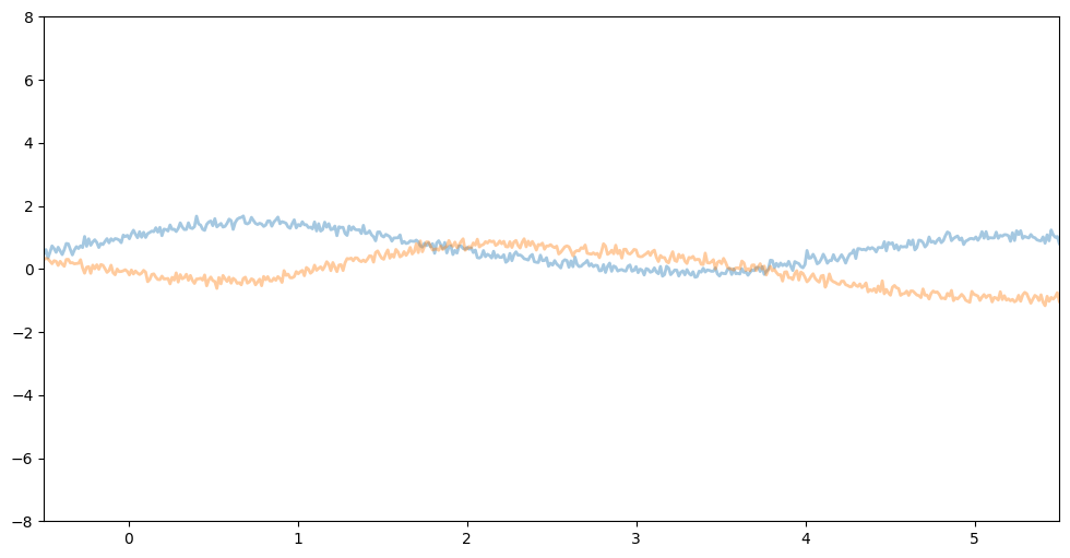
X = dist.Uniform(0.0, 5.0).sample(sample_shape=(N,))
y = 0.5 * torch.sin(3 * X) + dist.Normal(0.0, 0.2).sample(sample_shape=(N,))
plot(plot_observed_data=True)
5.3.3. Model Definition#
Beginning with the definition of the RBF kernel, we then construct a Gaussian Process regression object and sample from this prior without training it for our synthetic data.
kernel = gp.kernels.RBF(
    input_dim=1, variance=torch.tensor(6.0), lengthscale=torch.tensor(0.05)
)
gpr = gp.models.GPRegression(X, y, kernel, noise=torch.tensor(0.1))
plot(model=gpr, kernel=kernel, n_prior_samples=2)
_ = plt.ylim((-8, 8))
What would change if we increase the lengthscale? We will obtain much smoother function samples.
In reverse, this means that the shorter the lengthscale the more rugged our function samples are.
What happens if we reduce the variance and the noise? The vertical amplitude gets smaller and smaller.
In reverse, this means that the larger the variance and the noise, the larger the vertical amplitude of our function samples.
In examples:
kernel2 = gp.kernels.RBF(
    input_dim=1, variance=torch.tensor(6.0), lengthscale=torch.tensor(1)
)
gpr2 = gp.models.GPRegression(X, y, kernel2, noise=torch.tensor(0.1))
plot(model=gpr2, kernel=kernel2, n_prior_samples=2)
_ = plt.ylim((-8, 8))
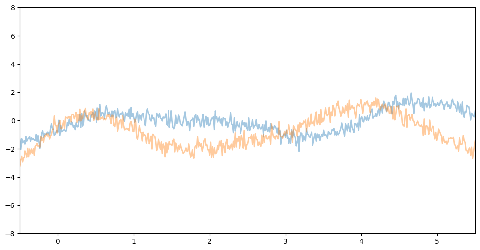
kernel3 = gp.kernels.RBF(
    input_dim=1, variance=torch.tensor(1.0), lengthscale=torch.tensor(1)
)
gpr3 = gp.models.GPRegression(X, y, kernel3, noise=torch.tensor(0.01))
plot(model=gpr3, kernel=kernel3, n_prior_samples=2)
_ = plt.ylim((-8, 8))
5.3.4. Inference#
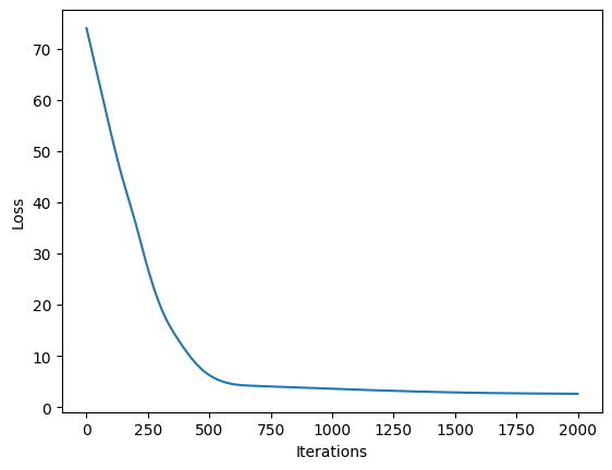
To now adjust the kernel hyperparameters to our synthetic data, we have to perform inference. For this we define the Evidence-Lower-Bound (ELBO) and construct a scenario in which we essentially perform gradient ascent on the log marginal likelihood, i.e. we computationally solve the Marginal Likelihood Estimation (MLE) to infer the right model parameters.
optimizer = torch.optim.Adam(gpr.parameters(), lr=0.005)
loss_fn = pyro.infer.Trace_ELBO().differentiable_loss
losses = []
variances = []
lengthscales = []
noises = []
num_steps = 2000
for i in range(num_steps):
    variances.append(gpr.kernel.variance.item())
    noises.append(gpr.noise.item())
    lengthscales.append(gpr.kernel.lengthscale.item())
    optimizer.zero_grad()
    loss = loss_fn(gpr.model, gpr.guide)
    loss.backward()
    optimizer.step()
    losses.append(loss.item())
Plotting the loss curve after 2000 training iterations
def plot_loss(loss):
    plt.plot(loss)
    plt.xlabel("Iterations")
    _ = plt.ylabel("Loss")  # supress output text


plot_loss(losses)
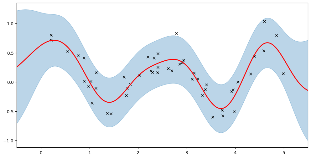
With that the behaviour of our Gaussian Process should now be much more reasonable, let’s inspect it
plot(model=gpr, plot_observed_data=True, plot_predictions=True)

In this plot we have the typical case of GP representation:
A, in this case red, line represents the mean prediction
A shaded area, in this case blue, represents the 2-sigma uncertainty around the mean
But what are the actual hyperparameters we just learned?
gpr.kernel.variance.item()
0.25187239303491094
gpr.kernel.lengthscale.item()
0.524795243437157
gpr.noise.item()
0.03603591991010109
The learning process can furthermore be illustrated for the GP’s behaviour across training iterations:
fig, ax = plt.subplots(figsize=(12, 6))


def update(iteration):
    pyro.clear_param_store()
    ax.cla()
    kernel_iter = gp.kernels.RBF(
        input_dim=1,
        variance=torch.tensor(variances[iteration]),
        lengthscale=torch.tensor(lengthscales[iteration]),
    )
    gpr_iter = gp.models.GPRegression(
        X, y, kernel_iter, noise=torch.tensor(noises[iteration])
    )
    plot(model=gpr_iter, plot_observed_data=True, plot_predictions=True, ax=ax)
    ax.set_title(f"Iteration: {iteration}, Loss: {losses[iteration]:0.2f}")


anim = FuncAnimation(fig, update, frames=np.arange(0, num_steps, 30), interval=100)
plt.close()

anim.save("../imgs/gpr-fit.gif", fps=60)
5.3.5. Maximum a Posteriory Estimation (MAP)#
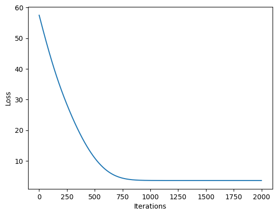
A second option is then to use MAP estimation for which we need to define priors over our hyperparameters to then infer the true hyperparameters.
pyro.clear_param_store()
kernel = gp.kernels.RBF(
    input_dim=1, variance=torch.tensor(5.0), lengthscale=torch.tensor(10.0)
)
gpr = gp.models.GPRegression(X, y, kernel, noise=torch.tensor(1.0))

# Define the priors over our hyperparameters
gpr.kernel.lengthscale = pyro.nn.PyroSample(dist.LogNormal(0.0, 1.0))
gpr.kernel.variance = pyro.nn.PyroSample(dist.LogNormal(0.0, 1.0))

optimizer = torch.optim.Adam(gpr.parameters(), lr=0.005)
loss_fn = pyro.infer.Trace_ELBO().differentiable_loss
losses = []
num_steps = 2000
for i in range(num_steps):
    optimizer.zero_grad()
    loss = loss_fn(gpr.model, gpr.guide)
    loss.backward()
    optimizer.step()
    losses.append(loss.item())

plot_loss(losses)
plot(model=gpr, plot_observed_data=True, plot_predictions=True)
What we then realize is that due to the priors we have defined, we end up with different hyperparameters than under the Maximum Likelihood Estimation (MLE)
gpr.set_mode("guide")
print("variance = {}".format(gpr.kernel.variance))
print("lengthscale = {}".format(gpr.kernel.lengthscale))
print("noise = {}".format(gpr.noise))
variance = 0.24541736830257171
lengthscale = 0.5144261073855972
noise = 0.035988066300649386
For the choice of prior we would ideally like to select parameters which maximise the model likelihood, which is defined by
For a single observation our likelihood would then be
We hence seek to maximise the likelihood, or the log-likelihood with respect to the kernel’s parameters in order to find the most well-suited prior. As priors encode our prior belief over the function to approximate, they are hugely important choices to make which later on determine the performance of our Gaussian process. The question one should hence ask in selecting kernels are:
Is my data stationary?
Is it differentiable, if so what is it’s regularity?
Do I expect any particular trends?
Do I expect periodicity, cycles, additivity, or other patterns?
5.3.6. Gaussian Process Classification#
To use Gaussian Processes for classification we first need to a softmax to our function prior
or going further
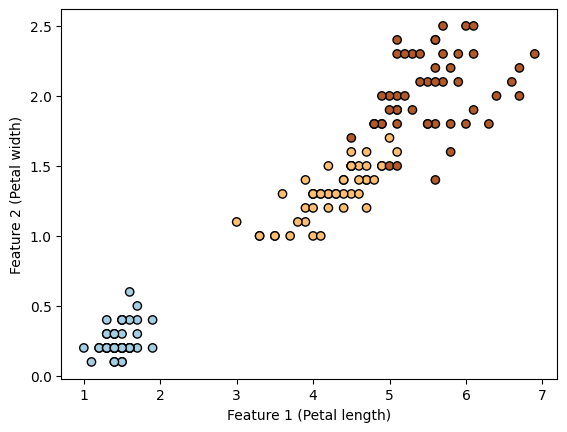
using one of Seaborn’s naturally provided datasets, the Iris dataset we can then construct a classification problem with 3 classes:
Setosa
Versicolor
Virginica
with just the petal length, and the petal width as input featurs.
df = sns.load_dataset("iris")
df.head()
| sepal_length | sepal_width | petal_length | petal_width | species | |
|---|---|---|---|---|---|
| 0 | 5.1 | 3.5 | 1.4 | 0.2 | setosa |
| 1 | 4.9 | 3.0 | 1.4 | 0.2 | setosa |
| 2 | 4.7 | 3.2 | 1.3 | 0.2 | setosa |
| 3 | 4.6 | 3.1 | 1.5 | 0.2 | setosa |
| 4 | 5.0 | 3.6 | 1.4 | 0.2 | setosa |
X = torch.from_numpy(
    df[df.columns[2:4]].values.astype("float32"),
)
df["species"] = df["species"].astype("category")
# encode the species as 0, 1, 2
y = torch.from_numpy(df["species"].cat.codes.values.copy())
plt.scatter(X[:, 0], X[:, 1], c=y, cmap=plt.cm.Paired, edgecolors=(0, 0, 0))
plt.xlabel("Feature 1 (Petal length)")
_ = plt.ylabel("Feature 2 (Petal width)")
Using the classical RBF-kernel
kernel = gp.kernels.RBF(input_dim=2)
pyro.clear_param_store()
likelihood = gp.likelihoods.MultiClass(num_classes=3)
# Important -- we need to add latent_shape argument here to the number of classes we have in the data
model = gp.models.VariationalGP(
X,
y,
kernel,
likelihood=likelihood,
whiten=True,
jitter=1e-03,
latent_shape=torch.Size([3]),
)
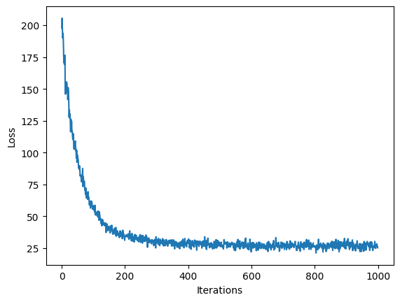
num_steps = 1000
loss = gp.util.train(model, num_steps=num_steps)
plot_loss(loss)
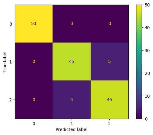
With which we can now inspect the accuracy of our classifier
mean, var = model(X)
y_hat = model.likelihood(mean, var)

print(f"Accuracy: {(y_hat==y).sum()*100/(len(y)) :0.2f}%")
Accuracy: 94.00%
And can furthermore use the confusion matrix to assess the accuracy of our predictions
cm = confusion_matrix(y, y_hat, labels=[0, 1, 2])
ConfusionMatrixDisplay(cm).plot()
<sklearn.metrics._plot.confusion_matrix.ConfusionMatrixDisplay at 0x32c50c7f0>
5.3.7. Gaussian Process Classification: The tl;dr#
Quickly summarizing GP classification (in a slightly different notation)
Based on the Bayesian methodology, where we have to assume an underlying prior distribution to guarantee smoothness with the final classifier then being a Bayesian classifier, which provides the best first for the observed data. The initial problem here is that our posterior is not directly Gaussian, as has to be presumed in a Gaussian process, i.e.
with the log-probability
We are then interested in the following moments of our probability distribution, which we first decompose as a conditional probability, i.e. \(p(f, y) = p(y|f)p(f)\)
\(Z\) is then used for hyperparameter tuning, \(\bar{f}\) gives us a point estimator, and \(\text{var}(f)\) is our error estimator. To gain a classification estimator with the Gaussian process estimator with the Gaussian Process framework, we have to utilize the Laplace approximation to gain a classification estimator. For the Gaussian Process framework we then have to find the maximum posterior probability for latent \(f\) at training points
by assigning approximate Gaussian posteriors at the training points
Our Laplace approximation \(q\) for the classification probability \(p\) is then given by
With which we can then compute the label probabilities
The Laplace approximation is only locally valid, working well within the logistic regression framework as the log posterior is concave and the structure of the link function yields an almost Gaussian posterior.
The training algorithm is then given by
and the prediction algorithm is given by
Gaussian classification does hence in summary amount to
The model outputs are modeled as transformations of latent functions with Gaussian priors
The non-Gaussian likelihood, the posterior is hence also non-Gaussian resulting in inference being intractable
This requires us to utilize Laplace approximations
With the Laplace approximations we then obtain Gaussian posteriors on training points
5.3.8. Combining Kernels#
Pyro provides utilities to combine the different kernels, the most important of which are shown by example below:
linear = gp.kernels.Linear(
    input_dim=1,
)
periodic = gp.kernels.Periodic(
    input_dim=1, period=torch.tensor(0.5), lengthscale=torch.tensor(4.0)
)
rbf = gp.kernels.RBF(
    input_dim=1, lengthscale=torch.tensor(0.5), variance=torch.tensor(0.5)
)
k1 = gp.kernels.Product(kern0=rbf, kern1=periodic)

k = gp.kernels.Sum(linear, k1)
5.4. Remarks#
If you have to apply Gaussian Processes to large datasets, or the training is too slow for your liking, take a look at Sparse Gaussian Processes. This class of Gaussian Processes seeks to avoid the computational constraints of traditional Gaussian Processes.
5.5. Tasks#
Methods of Inference and the Computational Cost of Methods
Explore the use of other inference methods to infer the hyperparameters of the Gaussian Processes Regression with Monte Carlo-style algorithms as you’ve encountered earlier in the course
Measure the difference in computational cost between the three approaches
Repeat the same task for Gaussian Process Classification
Kernel Choices
Experiment with the different combinations of the different kernels, visualize the combinations, and consider for which kind of function you would potentially use them
Inspect the performance of your constructed kernels for GP Regression
Repeat the same task for Gaussian Process Classification