12. Encoder-Decoder Models#
Learning outcome
How can one compress data in a linearly optimal way?
What is the meaning of the PCA principal components when applied to a dataset, and how can that be used to choose their count?
Draw the autoencoder architecture and explain when/why it is superior to linear compression.
A great many models in machine learning build on the Encoder-Decoder paradigm, but what is the intuition behind said paradigm? The core intuition is that while our original data may be high-dimensional, a good prediction only depends on a few key sub-dimensions of the original data, and as such, we can dimensionally reduce our original data through an Encoder before predicting or reconstructing our data onto the original data-plane with the Decoder.
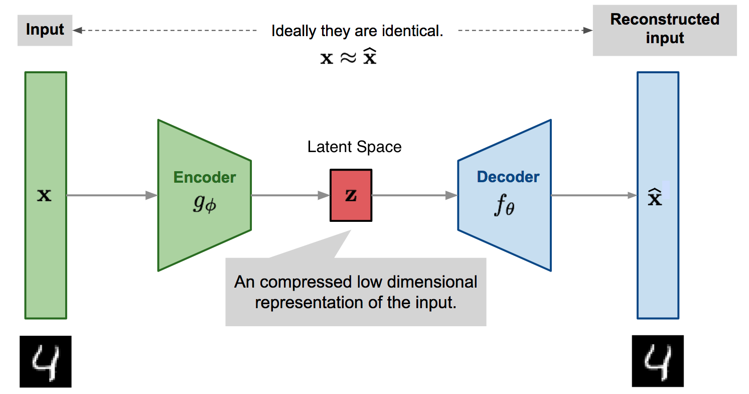
Fig. 12.1 Autoencoder architecture (Adapted from lilianweng.github.io).#
The precursor to this paradigm is the realization of which parameters/variables of our data are actually relevant. For this purpose, we look at its roots in computational linear algebra, beginning with the Singular Value Decomposition to build towards the Principal Component Analysis, which subsequently feeds into Autoencoder which is the epitome of the Encoder-Decoder paradigm and builds on the key insights from the Principal Component Analysis.
12.1. Singular Value Decomposition#
Generalizing the eigendecomposition of small matrices, the singular value decomposition allows for the factorization of real or complex matrices. For any matrix, this decomposition can be computed, but only square matrices with a full set of linearly independent eigenvectors can be diagonalized. Any \(A \in \mathbb{R}^{m \times n}\) can be factored as
where \(U \in \mathbb{R}^{m \times m}\) is a unitary matrix, where the columns are eigenvectors of \(A A^{\top}\), \(\Sigma\) is a diagonal matrix \(\Sigma \in \mathbb{R}^{m \times n}\), and \(V \in \mathbb{R}^{n \times n}\) is a unitary matrix whose columns are eigenvectors of \(A^{\top}A\). I.e.
where \(\sigma_{n}\) can also be 0. The singular values \(\sigma_{1} \geq \ldots \sigma_{r} \geq 0\) are square roots of the eigenvalues of \(A^{\top}A\), and \(r = \text{rank}(A)\).
if symmetric and has \(n\) real eigenvalues. Here \(V \in \mathbb{R}^{n \times n}\), columns are eigenvectors of \(A^{\top}A\), and \(D \in \mathbb{R}^{n \times n}\) is the diagonal matrix of real eigenvalues.
if symmetric, and real has \(m\) real eigenvalues. In this case, \(U \in \mathbb{R}^{m \times m}\) of which the columns are eigenvectors of \(AA^{\top}\), and \(D' \in \mathbb{R}^{m \times m}\) is a diagonal matrix of real eigenvalues. The geometric analogy of the singular value decomposition is then
\(A\) is a matrix of \(r = \text{rank}(A)\)
\(U\) is the rotation/reflection
\(\Sigma\) is the stretching
\(V^{\top}\) is the rotation/reflection
Broken down into its individual pieces, we get the following commutative diagram:
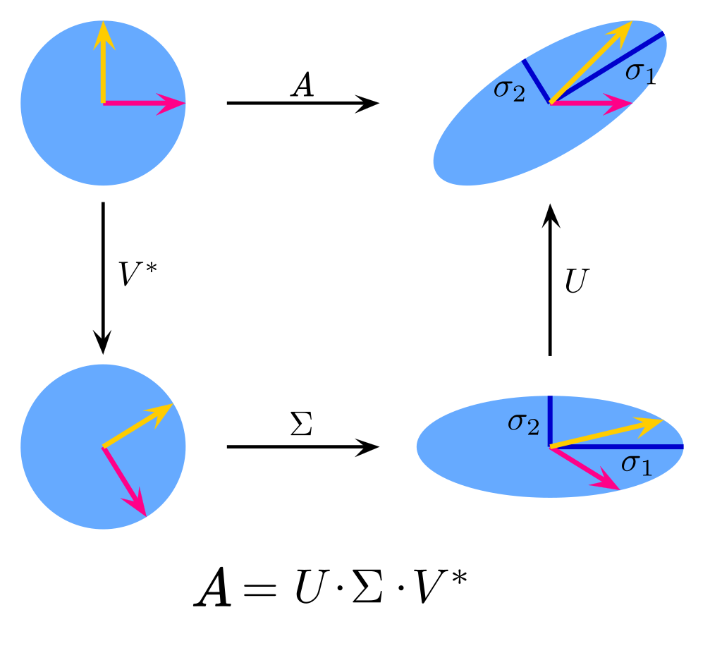
Fig. 12.2 Decomposing the effect of a matrix transforming a vector into its SVD components (Adapted from Wikipedia).#
The singular value decomposition of \(A\) can then be expressed in terms of a basis of \(\text{range}(A)\) and a basis of \(\text{range}(A^{\top})\).
where \(V\) is the eigenvector matrix (columns) of \(A^{\top}A\), and the large matrix \(\Sigma\) is a diagonal matrix of eigenvalues of \(A^{\top}A\). Also,
where \(U\) is the eigenvector matrix (columns) of \(A A^{\top}\), and the large diagonal matrix consists of the eigenvalues of \(A A^{\top}\). Graphically, this decomposition looks like this:
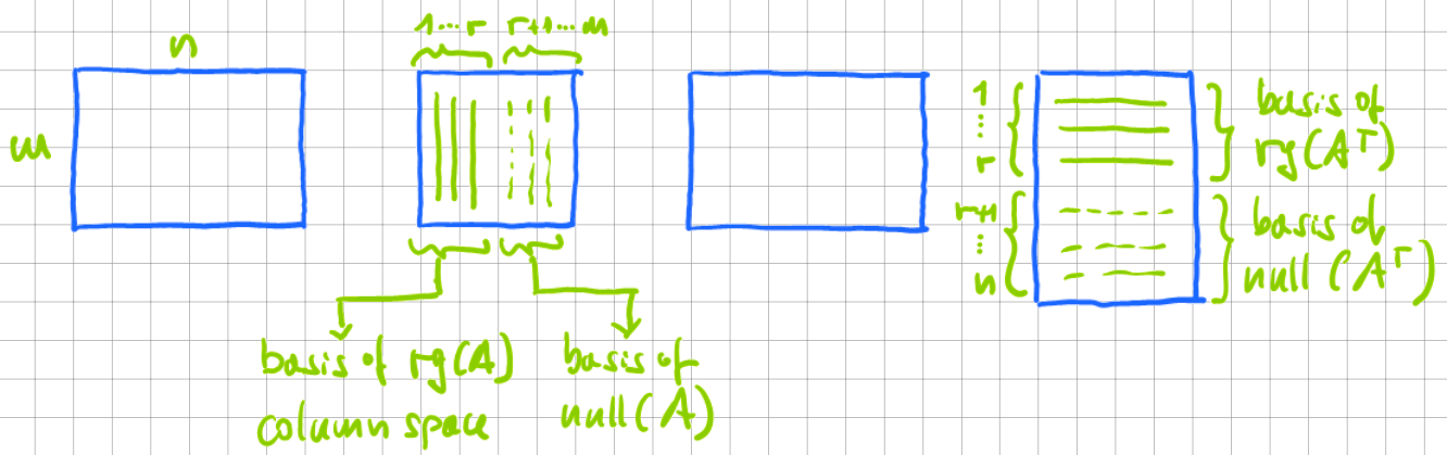
Fig. 12.3 Singular value decompositions of a matrix \(A=U\Sigma V^{\top}\). From left to right: \(A\), \(U\), \(\Sigma\), \(V^{\top}\).#
12.1.1. Advanced Topics: Moore-Penrose pseudo-inverse#
One application of singular value decomposition is to, e.g., compute the pseudo-inverse, also called the Moore-Penrose Inverse of a matrix \(A \in \mathbb{R}^{m \times n}\).
Given \(A \in \mathbb{R}\), \(x \in \mathbb{R}^{n}\), and \(y \in \mathbb{R}^{m}\), we consider the task of solving the following linear equation system for \(x\):
where \(y \notin \text{col}(A)\), i.e., not in the column space of A, is allowed.
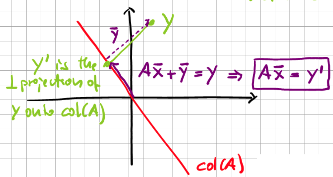
Fig. 12.4 Geometric interpretation of Moore-Penrose inverse.#
Here, \(y'\) is the orthogonal projection of \(y\) onto the column space of \(A\). With this transformation, we are transforming the problem to
which is exactly what we require the pseudo-inverse for, as it assures that the error \(|| \bar{y}|| = \min\) is minimal. We then employ the singular value decomposition of \(A\) to solve \(Ax=y\) in a least-squares sense:
where \(A^{+}\) is the pseudo-inverse with
As the approximation of \(x\), we then compute
If \(A\) is invertible \(\Rightarrow A^{+} = A^{-1} \Rightarrow \bar{x} = x\), and we obtain the exact solution.
If A is singular, and \(y \in \text{col}(A)\), then \(\bar{x}\) is the solution which minimizes \(||\bar{x}||_{2}\) as \(( \bar{x} + \text{null}(A))\), and all are possible solutions.
If A is singular, and \(y \notin \text{col}(A)\), then \(\bar{x}\) is the least-squares solution which minimizes \(|| A \bar{x} - y ||_{2}\)
Some useful properties of the pseudo-inverse are:
From which follows that \(A \in \mathbb{R}^{m \times n}\) with n linearly independent columns \(A^{\top}A\) is invertible. The following relations apply to \(A^{+}\):
12.2. Principal Component Analysis#
To further discern information in our data which is not required for our defined task, be it classification or regression, we can apply principal component analysis to reduce the dimensionality. Principal component analysis finds the optimal linear map from a \(D\)-dimensional input to the design matrix on a \(K\)-dimensional space. Expressing this relation in probabilistic terms, we speak of a linear map \(D \rightarrow K\) with maximum variance \(\Longrightarrow\) “autocorrelation” of the input data. This linear map can be written the following way in matrix notation:
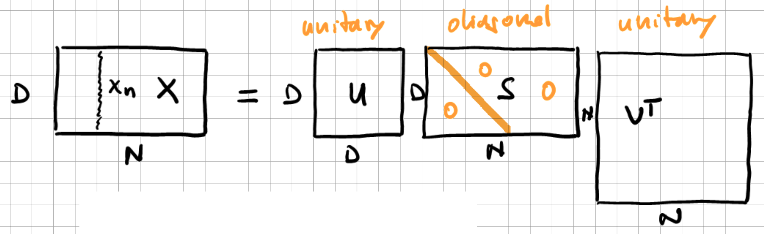
Fig. 12.5 SVD applied to dataset \(X\) of \(D\)-dimensional vectors \(x_n\).#
Here, \(U\) are the left singular vectors, \(S\) are the singular values, and \(V^{\top}\) are the right singular values. This dimensionality reduction is achieved through the singular value decomposition (SVD). What we seek to achieve is to compress
where the rank of \(\hat{x}\) is \(K\). To derive the relation between SVD and PCA, we can use the following Lemma:
Here, the \(s_{i}\) are the ordered singular values \(s_{1} \geq s_{2} \geq \ldots \geq 0\), and \(\tilde{U}\) is a \(D \times K\) matrix
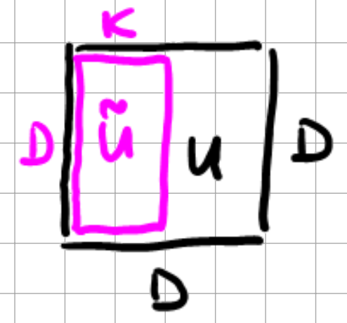
Fig. 12.6 \(\tilde{U}\) matrix.#
We then have
as we have
From a probabilistic view, we are creating N independent identically distributed (i.i.d) \(D\)-dimensional vectors \(x_{n}\), see the left side of Fig. 12.5. We then have a sample mean, sometimes called empirical mean, of
and a sample co-variance (biased), sometimes called empirical covariance, of
for \(N \rightarrow \infty\) the two then converge to
if we assume for simplicity that \(\bar{x} = 0\), then
where \(S^{(2)}\) is a newly constructed singular value matrix. Comparing this with the compressed matrix
from which follows
The data vectors \(\hat{x}_{n}\) in \(\hat{x}\) are hence uncorrelated, and \(\hat{x}_{1}\) has the highest variance by ordering the singular values. If you were to consider the case of classification, then the lesson of PCA is that data with higher variance is always better to classify, as it is the more important information contained in the dataset.
The number of principal components we consider is effectively a hyperparameter we must carefully evaluate before making a choice. See the reconstruction error on MNIST vs the number of latent dimensions used by the PCA as an example.
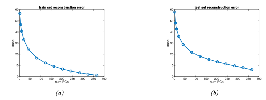
Fig. 12.7 Reconstruction error vs number of latent dimensions used by PCA (Souce: [Murphy, 2022]).#
With this all being a bit abstract, here are a few examples of applications of PCA to increasingly more practical applications.
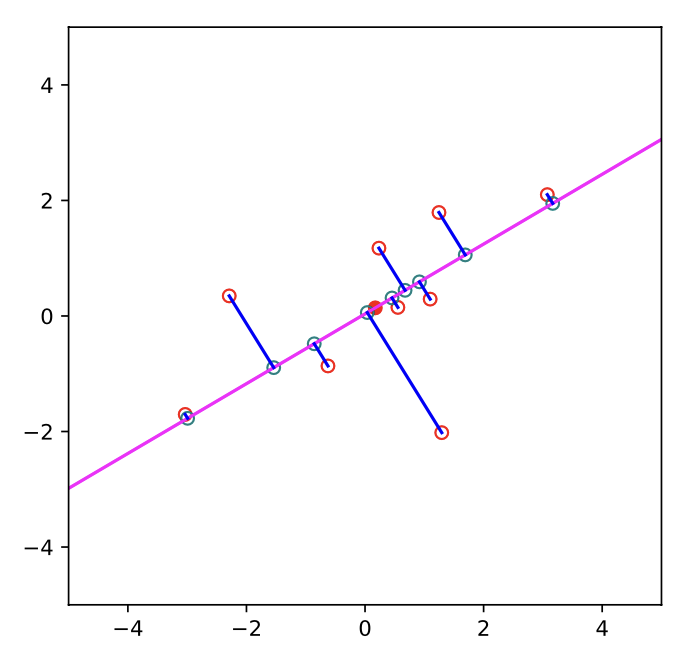
Fig. 12.8 PCA projection of 2d data onto 1d (Souce: [Murphy, 2022]).#
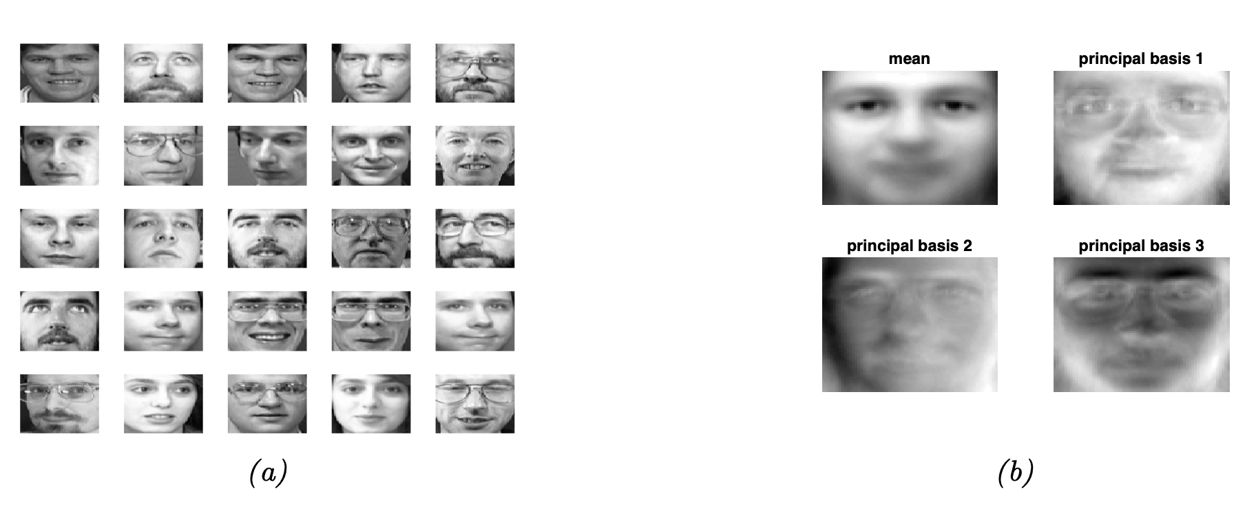
Fig. 12.9 (a) Randomly chosen images were taken from the Olivetti face database. (b) mean and first three PCA components (Souce: [Murphy, 2022]).#
12.2.1. Computational Issues of Principal Components Analysis#
So far, we have only considered the eigendecomposition of the covariance matrix, but computationally, the correlation matrix is more advantageous. This avoids the potential of a “confused” PCA due to a mismatch between length scales in the dataset.
12.3. Autoencoder#
These dimensionality reduction techniques originating from computational linear algebra led to the construction of Autoencoders in machine learning, an encoder-decoder network focussed solely on the reconstruction error of a network-induced dimensionality reduction in the classical case. Considering the linear case, we have the following network:
with \(W_{1} \in \mathbb{R}^{L \times D}\), \(W_{2} \in \mathbb{R}^{D \times L}\), and \(L < D\). This network can hence be simplified as \(\hat{x} = W_{2}W_{1}x = Wx\) as the output of the model. The autoencoder is trained for the reconstruction error
which results in \(\hat{W}\) being an orthogonal projection onto the first L eigenvectors of the empirical covariance of the data. Hence is equivalent to performing PCA. This is where the real power of the autoencoder begins, as it can be extended in many directions:
Addition of nonlinearities
More and deeper layers
Usage of specialized architectures like convolutions for more efficient computation
There are no set limits to the addition of further quirks here.
12.4. Further References#
[Murphy, 2022], 20.1 PCA and 20.3 Autoencoders