1. Linear Models

1.1. Linear Regression

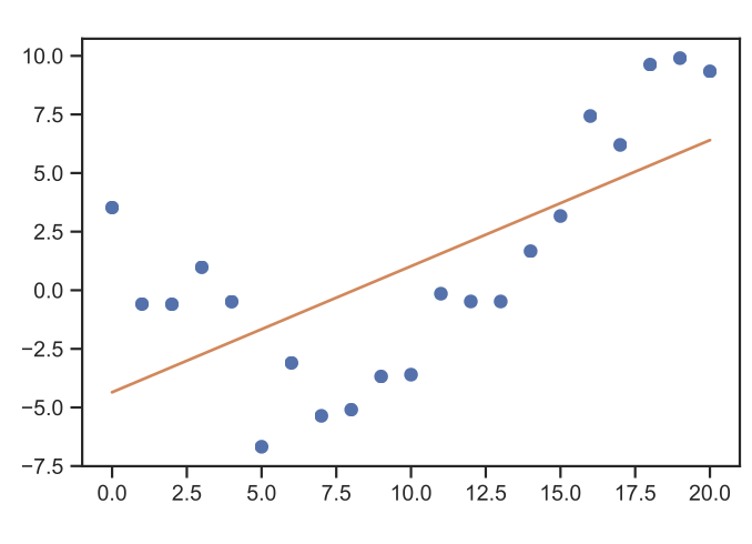
Linear regression belongs to the family of supervised learning approaches, as it inherently requires labeled data. With it being the simplest regression approach. The simplest example to think of would be “Given measurement pairs \(\left\{(x^{(i)}, y^{(i)})\right\}_{i=1,...m}\), how to fit a line \(h(x)\) to best approximate \(y\)?”

Do you remember this from last lecture?

How does it work?

1. We begin by formulating a hypothesis for the relation between input \(x \in \mathbb{R}^{n}\), and output \(y \in \mathbb{R}^{p}\). For conceptual clarity, we will initially set \(p=1\). Then our hypothesis is represented by

   (1.1)\[h(x)=\vartheta^{\top} x, \quad h \in \mathbb{R} \qquad(\text{more generally, } h \in \mathbb{R}^p),\]

   where \(\vartheta \in \mathbb{R}^{n}\) are the parameters of our hypothesis. To add an offset to this linear model, we could assume that the actual dimension of \(x\) is \(n-1\), and we add a dummy dimension of ones to \(x\) (see Exercise 1 for more details).

2. Then we need a strategy to fit our hypothesis parameters \(\vartheta\) to the data points we have \(\left\{(x^{(i)}, y^{\text {(i)}})\right\}_{i=1,...m}\).

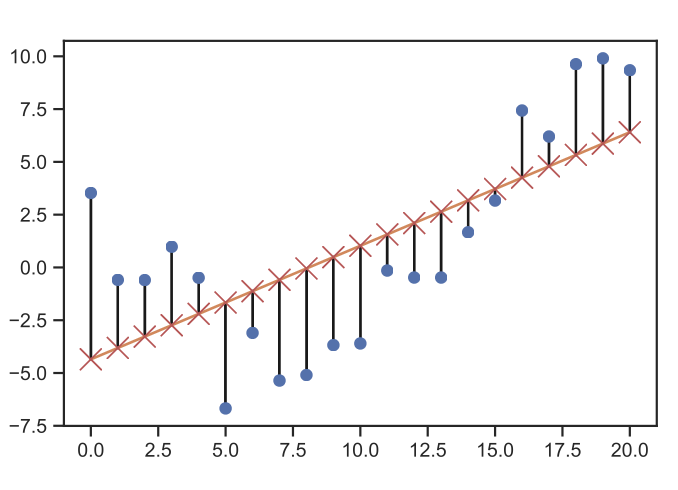
   1. Define a suitable cost function \(J\), which emphasizes the importance of certain traits to the model. I.e. if a certain data area is of special importance to our model we should penalize modeling failures for those points much more heavily than others. A typical choice is the Least Mean Square (LMS) i.e.

      (1.2)\[J(\vartheta)=\frac{1}{2} \sum_{i=1}^{m}\left(h(x^{(i)})-y^{(i)}\right)^{2}\]

   2. Through an iterative application of gradient descent (more on this later in the course) find a \(\vartheta\) which minimizes the cost function \(J(\vartheta)\). If we apply gradient descent, our update function for the hypothesis parameters then takes the following shape

   (1.3)\[\vartheta^{(k+1)}=\vartheta^{(k)}-\alpha\frac{\partial J}{\partial \vartheta^{k}}.\]

The iteration scheme can then be computed as:

(1.4)\[\begin{split} \begin{aligned} \frac{\partial J}{\partial \vartheta_{j}}&=\frac{\partial}{\partial \vartheta_{j}} \frac{1}{2} \sum_{i}\left(h(x^{(i)})-y^{(i)}\right)^{2} \\ &=\underset{i}{\sum} \left(h(x^{(i)})-y^{(i)}\right) \frac{\partial }{\partial \vartheta_{j}}\left(h(x^{(i)})-y^{(i)}\right) \\ &=\sum_{i}\left(h(x^{(i)})-y^{(i)}\right) x_{j}^{(i)}. \end{aligned} \end{split}\]

Resubstituting the iteration scheme into the update function, we then obtain the formula for batch gradient descent

(1.5)\[\vartheta^{(k+1)}_j=\vartheta^{(k)}_j-\alpha\sum_{i=1}^m\left(h^{(k)}(x^{(i)})-y^{(i)}\right) x_{j}^{(i)}, \qquad (\text{for every }j).\]

We can choose to use randomly drawn subsets of all \(m\) data points at each iteration step, and then we call the method stochastic gradient descent.

1.1.1. Analytical Solution

If we now utilize matrix-vector calculus, then we can find the optimal \(\vartheta\) in one shot. To do this, we begin by defining our design matrix \(X\)

(1.6)\[\begin{split}X_{m \times n}=\left[\begin{array}{c}x^{(1) \top }\\ \vdots \\ x^{(i) \top} \\ \vdots \\ x^{(m) \top}\end{array}\right].\end{split}\]

and then define the feature vector from all samples as

(1.7)\[\begin{split}Y_{m \times 1}=\left[\begin{array}{c}y^{(1)} \\ \vdots \\ y^{(i)} \\ \vdots \\ y^{(m)}\end{array}\right].\end{split}\]

Connecting the individual pieces we then get the update function as

(1.8)\[\begin{split}X \vartheta _ {n\times 1} -Y = \left[\begin{array}{c} h(x^{(0)})-y^{(1)} \\ \vdots \\ h(x^{(i)})-y^{(i)} \\ \vdots \\ h(x^{(m)})-y^{(m)} \end{array}\right].\end{split}\]

According to which, the cost function then becomes

(1.9)\[J(\vartheta)=\frac{1}{2}(X \vartheta-Y)^{\top}(X \vartheta-Y).\]

As our cost function \(J(\vartheta)\) is convex, we now only need to check that there exists a minimum, i.e.

(1.10)\[\nabla_{\vartheta} J(\vartheta) \stackrel{!}{=} 0.\]

Computing the derivative

(1.11)\[\begin{split}\begin{align} \nabla_{\vartheta} J(\vartheta)&=\frac{1}{2} \nabla_{\vartheta}(X \vartheta-Y)^{\top}(X \vartheta-Y) \\ & =\frac{1}{2} \nabla_{\vartheta}(\underbrace{\vartheta^{\top} X^{\top} X \vartheta-\vartheta^{\top} X^{\top} Y-Y^{\top} X \vartheta}_{\text {this is in fact a scalar for $p=1$}}+Y^{\top} Y)\\ &=\frac{1}{2}\left(2X^{\top} X \vartheta-2 X^{\top} Y\right) \qquad (\text{use } {\nabla}_{\vartheta} Y^{\top} Y=0) \\ &=X^{\top} X \vartheta-X^{\top} Y \stackrel{!}{=} 0. \end{align} \end{split}\]

From which follows

(1.12)\[\begin{split} \begin{align} \Rightarrow & \quad X^{\top} X \vartheta=X^{\top} Y \\ \Rightarrow &\quad\vartheta=\left(X^{\top}X\right)^{-1}X^{\top}Y \end{align} \end{split}\]

How do we know that we are at a minumum and not a miximum? In the case of scalar intput \(x\in\mathbb{R}\), the second derivative of the error function \(\Delta_{\vartheta}J(\vartheta)\) becomes \(X^2\ge0\), which guarantees that the extremum is a minimum.

Exercise: Linear Regression Implementations

Implement the three approaches (batch gradient descent, stochastic gradient descent, and the matrix approach) to linear regression and compare their performance.

1. Batch Gradient Descent

2. Stochastic Gradient Descent

3. Matrix Approach

1.1.2. Probabilistic Interpretation

With much data in practice, having errors over the collected data itself, we want to be able to include a data error in our linear regression. The approach for this is Maximum Likelihood Estimation as introduced in the Introduction lecture. I.e. this means data points are modeled as

(1.13)\[y^{(i)}=\vartheta^{\top} x^{(i)}+\varepsilon^{(i)}\]

Presuming that all our data points are independent, identically distributed (i.i.d) random variables. The noise is modeled with a normal distribution

(1.14)\[p(\varepsilon^{(i)})=\frac{1}{\sqrt{2 \pi \sigma^{2}}} \exp{\left(-\frac{\varepsilon^{(i) 2}}{2 \sigma^{2}}\right)}.\]

While most noise distributions in practice are not normal, the normal (a.k.a. Gaussian) distribution has many nice theoretical properties making it much friendlier for theoretical derivations.

Using the data error assumption, we can now derive the probability density function (pdf) for the data

(1.15)\[p(y^{(i)} \mid x^{(i)} ; \vartheta)=\frac{1}{\sqrt{2 \pi \sigma^{2}}} \exp{\left({-\frac{\left(y^{(i)}-\vartheta^{\top} x^{(i)}\right)^{2}}{2\sigma^{2}}}\right)}\]

where \(y^{(i)}\) is conditioned on \(x^{(i)}\). If we now consider not just the individual sample \(i\), but the entire dataset, we can define the likelihood for our hypothesis parameters as

(1.16)\[\begin{split} \begin{align} L(\vartheta) &=p(Y \mid X ; \vartheta)=\prod_{i=1}^{m} p(y^{(i)} \mid x^{(i)} ; \vartheta) \\ &=\prod_{i=1}^{m} \frac{1}{\sqrt{2 \pi \sigma^{2}}} \exp{\left(-\frac{\left(y^{(i)}-\vartheta^{\top} x^{(i)}\right)^{2}}{2 \sigma^{2}}\right)} \end{align} \end{split}\]

The probabilistic strategy to determine the optimal hypothesis parameters \(\vartheta\) is then the maximum likelihood approach for which we resort to the log-likelihood as it is monotonically increasing, and easier to optimize for.

(1.17)\[\begin{split} \begin{aligned} l(\vartheta)&=\log L(\vartheta)=\log \prod_{i=1}^{m} \frac{1}{\sqrt{2 \pi \sigma^{2}}} \exp{\left(-\frac{\left(y^{(i)}-\vartheta^{\top} x^{(i)}\right)^{2}}{2 \sigma^{2}}\right)}\\ &=\sum_{i=1}^{m} \log \frac{1}{\sqrt{2 \pi \sigma^{2}}} \exp{\left(- \frac{\left(y^{(i)}-\vartheta^{\top} x^{(i)}\right)^{2}}{2 \sigma^{2}}\right)}\\ &=m \log \frac{1}{\sqrt{2 \pi \sigma^{2}}}-\frac{1}{2 \sigma^{2}} \sum_{i=1}^{m}\left(y^{(i)}-\vartheta^{\top} x^{(i)}\right)^{2}\\ \end{aligned} \end{split}\]

(1.18)\[ \Rightarrow \vartheta=\underset{\vartheta}{\arg \max}\; l(\vartheta)=\underset{\vartheta}{\arg \min} \sum_{i=1}^{m}\left(y^{(i)}-\vartheta^{\top} x^{(i)}\right)^{2} \]

This is the same result as minimizing \(J(\vartheta)\) from before. Interestingly enough, the Gaussian i.i.d. noise used in the maximum likelihood approach is entirely independent of \(\sigma^{2}\).

Least mean squares (LMS) method, as well as maximum likelihood regression as above are parametric learning algorithms.

If the number of parameters is not known beforehand, then the algorithms become non-parametric learning algorithms.

Can maximum likelihood estimation (MLE) be made more non-parametric? Following intuition, the linear MLE as well as the LMS critically depend on the selection of the features, i.e the dimension of the parameter vector \(\vartheta\). I.e. when the dimension of \(\vartheta\) is too low we tend to underfit, where we do not capture some of the structure of our data (more on under- and overfitting in Core Content 2). An approach called locally weighted linear regression (LWR) copes with the problem of underfitting by giving more weight to new, unseen query points \(\tilde{x}\). E.g. for \(\tilde{x}\), where we want to estimate \(y\) by \(h(\tilde{x})=\vartheta \tilde{x}\), we solve

(1.19)\[\vartheta=\underset{\vartheta}{\arg \min} \sum_{i=1}^{m} w^{(i)}\left(y^{(i)}-\vartheta^{\top} x^{(i)}\right)^{2},\]

where the weights \(\omega\) are given by

(1.20)\[\omega^{(i)}=\exp{\left(-\frac{\left(x^{(i)}-\tilde{x}\right)^{2}}{2 \tau^{2}}\right)},\]

with \(\tau\) being a hyperparameter. This approach naturally gives more weight to new datapoints. Hence making \(\vartheta\) crucially depend on \(\tilde{x}\), and making it more non-parametric.

1.2. Classification & Logistic Regression

Summarizing the differences between regression and classification:

Regression	Classification
\(x \in \mathbb{R}^{n}\)	\(x \in \mathbb{R}^{n}\)
\(y \in \mathbb{R}\)	\(y \in\{0,1\}\)

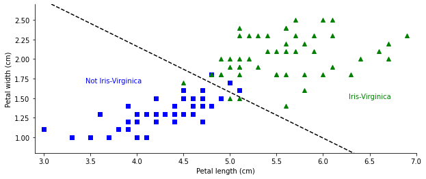
Fig. 1.1 Linear classification example. (Source: [Murphy, 2022], iris_logreg.ipynb)

To achieve such classification ability we have to introduce a new hypothesis function \(h(x)\). A reasonable choice would be to model the probability that \(y=1\) given \(x\) with a function \(h:\mathbb{R}\rightarrow [0,1]\). In the logistic regression approach

(1.21)\[ h(x) = \varphi ( \vartheta^{\top} x ) = \frac{1}{1+e^{-\vartheta^{\top} x}}, \]

where

(1.22)\[\varphi(x)=\frac{1}{1+e^{-x}}=\frac{1}{2}\left(1+\tanh\frac{x}{2}\right)\]

is the logistic function, also called the sigmoid function.

Fig. 1.2 Sigmoid function. (Source: Wikipedia)

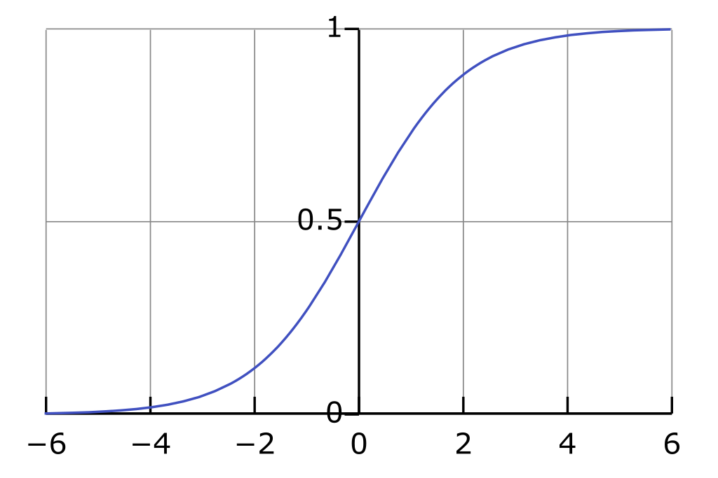
The advantage of this function lies in its many nice properties, such as its derivative:

(1.23)\[\varphi^{\prime} (x)=\frac{-1}{(1+e^{-x})^2} e^{-x}\cdot(-1)=\frac{1}{1+e^{-x}}\left(1-\frac{1}{1+e^{-x}}\right)=\varphi(x)(1-\varphi(x)).\]

If we now want to apply the Maximum Likelihood Estimation approach, then we need to use our hypothesis to assign probabilities to the discrete events

(1.24)\[\begin{split}\begin{cases}p(y=1 \mid x ; \vartheta)=h(x), & \\ p(y=0 \mid x ; \vartheta)=1-h(x). & \end{cases}\end{split}\]

This probability mass function corresponds to the Bernoiulli distribution and can be equivalently written as

(1.25)\[p(y \mid x ; \vartheta)=\left(h(x)\right)^{y}(1-h(x))^{1-y}.\]

This will look quite different for other types of labels, so be cautious in just copying this form of the pdf!

With our pdf we can then again construct the likelihood function

(1.26)\[L(\vartheta) = p(y | x ; \vartheta) =\prod_{i=1}^{m} p\left(y^{(i)} \mid x^{(i)}; \vartheta\right).\]

Assuming the previously presumed classification buckets, and that the data is i.i.d.

(1.27)\[ L(\vartheta)=\prod_{i=1}^{m} \left(h(x^{(i)})\right)^{y^{(i)}}\left(1-h(x^{(i)})\right)^{1-y^{(i)}}, \]

and then the log-likelihood decomposes to

(1.28)\[ l(\vartheta)=\log L(\vartheta)=\sum_{i=1}^{m}y^{(i)} \log h(x^{(i)})+(1-y^{(i)}) \log (1-h(x^{(i)})). \]

Again we can find \(\arg\max l(\vartheta)\) e.g. by gradient ascent (batch or stochastic):

(1.29)\[\vartheta_{j}^{(k+1)}=\vartheta_{j}^{(k)}+\left.\alpha \frac{\partial l(\vartheta)}{\partial \vartheta}\right|^{(k)}\]

(1.30)\[\begin{split}\begin{align} \frac{\partial \ell(\vartheta)}{\partial \vartheta_j} &=\sum_{i=1}^m\left(y^{(i)} \frac{1}{h(x^{(i)})}-(1-y^{(i)}) \frac{1}{1-h(x^{(i)})}\right) \frac{\partial h(x^{(i)})}{\partial \vartheta_j }\\ &=\sum_{i=1}^m\left(\frac{y^{(i)}-h(x^{(i)})}{h(x^{(i)})(1-h(x^{(i)}))}\right) h (x^{(i)})(1-h (x^{(i)})) x_j^{(i)}\\ &=\sum_{i=1}^m(y^{(i)}- h(x^{(i)})) x_j^{(i)} \end{align}\end{split}\]

(1.31)\[\Rightarrow \vartheta_{j}^{(k+1)}=\vartheta_{j}^{(k)}+\alpha \sum_{i=1}^m\left( y^{(i)}-h^{(k)}(x^{(i)}) \right) x_j^{(i)},\]

which we can then solve with either batch gradient descent or stochastic gradient descent.

Exercise: Vanilla Indicator (Perceptron)

Using the “vanilla” indicator function instead of the sigmoid:

(1.32)\[\begin{split} g(x)= \begin{cases}1, & x \geqslant 0 \\ 0, & x<0\end{cases} \end{split}\]

derive the update functions for the gradient methods, as well as the Maximum Likelihood Estimator approach.

1.3. Further References

Linear & Logistic Regression

• [Ng, 2022], Chapters 1 and 2 - main reference

• Machine Learning Basics video and slides from I2DL by Matthias Niessner (TUM).

• What happens if a linear regression is underdetermined i.e. we have fewer observations than parameters?