7. Gaussian Processes#
Learning outcome
How do Gaussian processes relate to the conditional Gaussian distribution?
What are valid ways to combine kernels?
Which hyperparameters describe a Gaussian process, and how do you tune them?
As the main mathematical construct behind Gaussian Processes, we first introduce the Multivariate Gaussian distribution. We analyze this distribution in some more detail to provide reference results. For a more detailed derivation of the results, refer to [Bishop, 2006], Section 2.3. In the rest of this lecture, we define the Gaussian Process and how it can be applied to regression and classification.
7.1. Multivariate Gaussian Distribution#
The univariate (for a scalar random variable) Gaussian distribution has the form
The two parameters are the mean \(\mu\) and variance \(\sigma^2\).
The multivariate Gaussian distribution then has the following form
with
\(x \in \mathbb{R}^d \quad \) - feature / sample / random vector
\(\mu \in \mathbb{R}^d \quad \) - mean vector
\(\Sigma \in \mathbb{R}^{d \times d} \quad\) - covariance matrix
Properties:
\(\Delta^2=(x-\mu)^{\top}\Sigma^{-1}(x-\mu)\) is a quadratic form.
\(\Delta\) is the Mahalanobis distance from \(\mu\) to \(x\). It collapses to the Euclidean distance for \(\Sigma = I\).
\(\Sigma\) is a symmetric positive definite matrix (i.e., its eigenvalues are strictly positive), and its diagonal elements contain the variance, i.e., covariance with itself.
\(\Sigma\) can be diagonalized with real eigenvalues \(\lambda_i\) and the corresponding eigenvectors \(u_i\) can be chosen to form an orthonormal set.
We construct the orthogonal matrix \(U\) as follows.
which fulfills
where \(\lambda\) denotes a diagonal matrix of eigenvalues. If we apply the variable transformation \(y=U(x-\mu)\), we can transform the Gaussian PDF of \(x\) to the \(y\) coordinates according to the change of variables rule (see the beginning of Gaussian Mixture Models).
which leads to
Note that the diagonalization of \(\Delta\) leads to a factorization of the PDF into \(d\) 1D PDFs.
7.1.1. 1st and 2nd Moment#
7.1.2. Conditional Gaussian PDF#
Consider the case \(x \sim \mathcal{N}(x; \mu, \Sigma)\) being a \(d\)-dimensional Gaussian random vector. We can partition \(x\) into two disjoint subsets \(x_a\) and \(x_b\).
The corresponding partitions of the mean vector \(\mu\) and covariance matrix \(\Sigma\) become
Note that \(\Sigma^T=\Sigma\) implies that \(\Sigma_{a a}\) and \(\Sigma_{b b}\) are symmetric, while \(\Sigma_{b a}=\Sigma_{a b}^{\mathrm{T}}\).
We also define the precision matrix \(\Lambda = \Sigma^{-1}\), being the inverse of the covariance matrix, where
and \(\Lambda_{a a}\) and \(\Lambda_{b b}\) are symmetric, while \(\Lambda_{a b}^{\mathrm{T}}=\Lambda_{b a}\). Note, \(\Lambda_{a a}\) is not simply the inverse of \(\Sigma_{a a}\).
Now, we want to evaluate \(\mathcal{N}(x_a| x_b; \mu, \Sigma)\) and use \(p(x_a, x_b) = p(x_a|x_b)p(x_b)\). We expand all terms of the pdf given the split considering all terms that do not involve \(x_a\) as constant, and then compare with the generic form of a Gaussian for \(p(x_a| x_b)\). We can decompose the equation into quadratic, linear, and constant terms in \(x_a\) and find an expression for \(p(x_a|x_b)\).
For all intermediate steps refer to [Bishop, 2006].
7.1.3. Marginal Gaussian PDF#
For the marginal PDF, we integrate out the dependence on \(x_b\) of the joint PDF:
We can follow similar steps as above for separating terms that involve \(x_a\) and \(x_b\). After integrating out the Gaussian with a quadratic term depending on \(x_b\) we are left with a lengthy term involving \(x_a\) only. By comparison with a Gaussian PDF and re-using the block relation between \(\Lambda\) and \(\Sigma\) as above, we obtain the marginal
7.1.4. Bayes Theorem for Gaussian Variables#
Generative learning addresses the problem of finding a posterior PDF from a likelihood and prior. The basis is Bayes rule for conditional probabilities
We want to find the posterior \(p(x|y)\) and the evidence \(p(y)\) under the assumption that the likelihood \(p(y|x)\) and the prior are linear Gaussian models.
\(p(y|x)\) is Gaussian and has a mean that depends at most linearly on \(x\) and a variance that is independent of \(x\).
\(p(x)\) is Gaussian.
These requirements correspond to the following structure of \(p(x)\) and \(p(y|x)\)
From that, we can derive an analytical evidence (marginal) and posterior (conditional) distributions (for more details see [Bishop, 2006]):
where
7.1.5. Maximum Likelihood for Gaussians#
In generative learning, we need to infer PDFs from data. Given a dataset \(X=(x_1, ..., x_N)\), where \(x_i\) are i.i.d. random variables drawn from a multivariate Gaussian, we can estimate \(\mu\) and \(\Sigma\) from the maximum likelihood (ML) (for more details see Bishop, 2006):
\(\mu_{ML}\) and \(\Sigma_{ML}\) correspond to the so-called sample or empirical estimates. However, \(\Sigma_{ML}\) does not deliver an unbiased estimate of the covariance if we use \(\mu_{ML}\) as \(\mu\). The difference decreases with \(N \to \infty\), but for a low \(N\), we have \(\Sigma_{ML} < \Sigma\). The practical reason for the discrepancy is that we use \(\mu_{ML}\) to estimate the mean, but this may not be the true mean. An unbiased sample variance can be defined using Bessel’s correction:
7.2. The Gaussian Process (GP)#
Gaussian Processes are a generalization of the generative learning concept based on Bayes rule and Gaussian distributions as models derived from Gaussian Discriminant Analysis. We explain Gaussian Processes (GPs) on the example of regression and discuss an adaptation to discrimination in the spirit of Gaussian Discriminant Analysis (GDA), however not being identical to GDA at the same time. Consider linear regression:
with \(\omega \in \mathbb{R}^{m}\) being the weights, \(\varphi \in \mathbb{R}^{m}\) the feature map, and \(h(x)\) the hypothesis giving the probability of \(y\). We now introduce an isotropic Gaussian prior on \(\omega\), where isotropic is defined as having a diagonal covariance matrix \(\Sigma\) with some scalar \(\alpha^{-1}\)
where \(0\) is the zero-mean nature of the Gaussian prior, with covariance \(\alpha^{-1} I\).
Note that \(\alpha\) is a hyperparameter, i.e. responsible for the model properties, it is called hyper \(\ldots\) to differentiate from the weight parameters \(\omega\).
Now let’s consider the data samples \(\left( y^{(i)} \in \mathbb{R}, x^{(i)} \in \mathbb{R}^{m} \right)_{i=1, \ldots, n}\). We are interested in leveraging the information contained in the data samples, i.e., in probabilistic lingo, the joint distribution of \(y^{(1)}, \ldots, y^{(n)}\). We can then write
where \(y \in \mathbb{R}^{n}\), \(\Phi \in \mathbb{R}^{n \times m}\), and \(\omega \in \mathbb{R}^{m}\). \(\Phi\) is the well-known design matrix from the lecture on Support Vector Machines, Eq. (6.58). As we know that \(\omega\) is Gaussian, the probability density function (pdf) of \(y\) is also Gaussian:
where \(K\) is the Grammian matrix we encountered in the SVM lecture.
A Gaussian Process is now defined as:
\(y^{(i)} = h(x^{(i)}), \; i=1, \ldots, n\) have a joint Gaussian PDF, i.e. are fully determined by their 2nd-order statistics (mean and covariance).
7.3. GP for Regression#
Take into account Gaussian noise on sample data as a modeling assumption:
for an isotropic Gaussian with precision parameter \(\beta\).
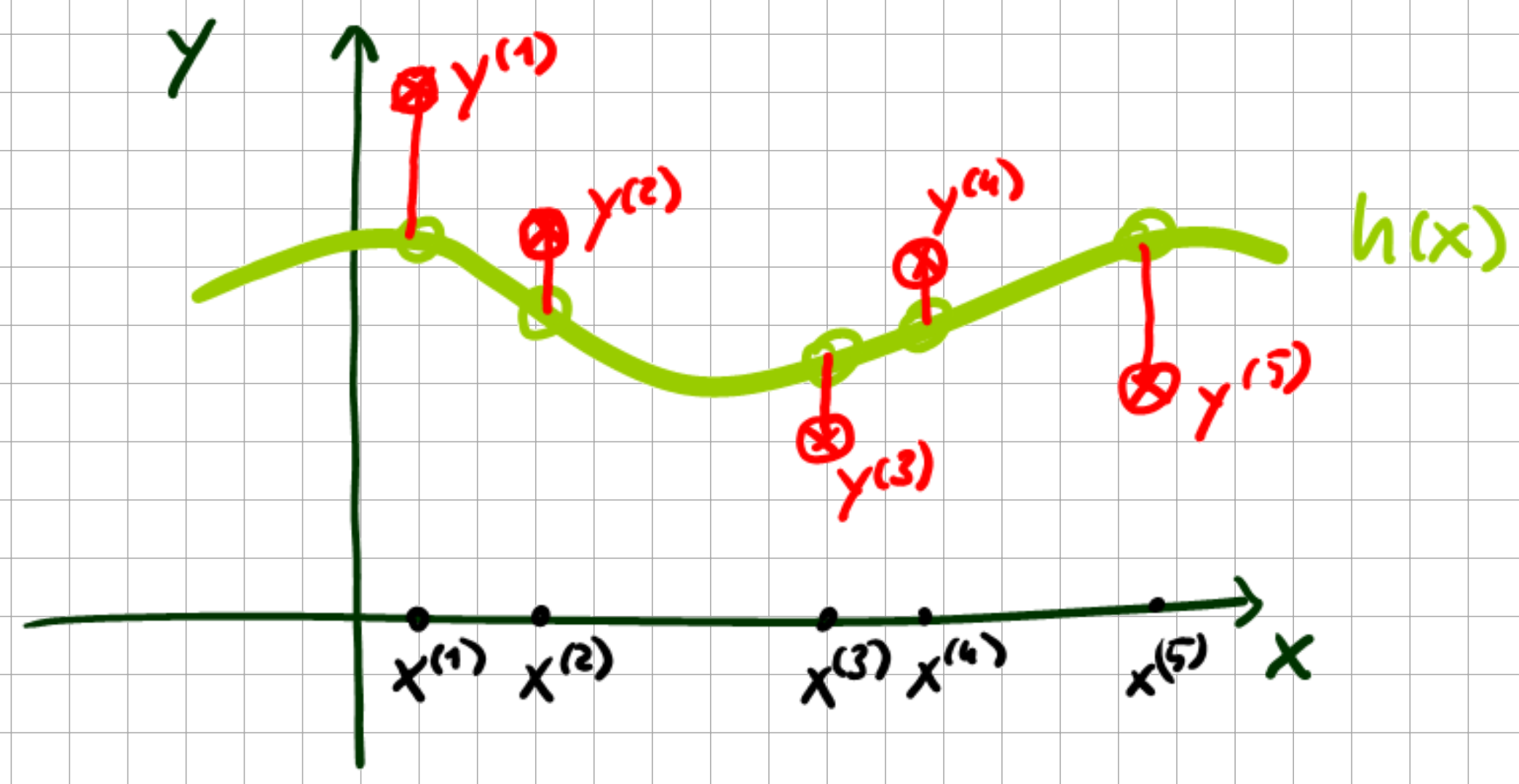
Fig. 7.1 Regression example.#
Here, \(h(x^{(i)}) = h^{(i)}\) becomes a latent variable. For the latent variables (these correspond to the noise-free regression data we considered earlier), we then obtain a Gaussian marginal PDF with some Grammatrix \(K\).
The kernel function underlying \(K\) defines a similarity such that if \(x_i\) and \(x_j\) are similar, then \(h(x_i)\) and \(h(x_j)\) should also be similar. The requisite posterior PDF then becomes
i.e. the posterior pdf is defined by the marginalization of \(p(y, h| x)\) over the latent variable \(h\). For the computation of \(p(y|x)\) we follow previous computations with adjustments of the notation where appropriate. We define the joint random variable \(z\) as
From Eq. (7.20) with prior \(p(h)\) and likelihood \(p(y|h)\) we recall that the evidence follows
into which we now substitute
Note that the kernel \(K\) can be presumed and is responsible for the prediction accuracy by the posterior. There exists a whole plethora of possible choices of K, the most common of which are:
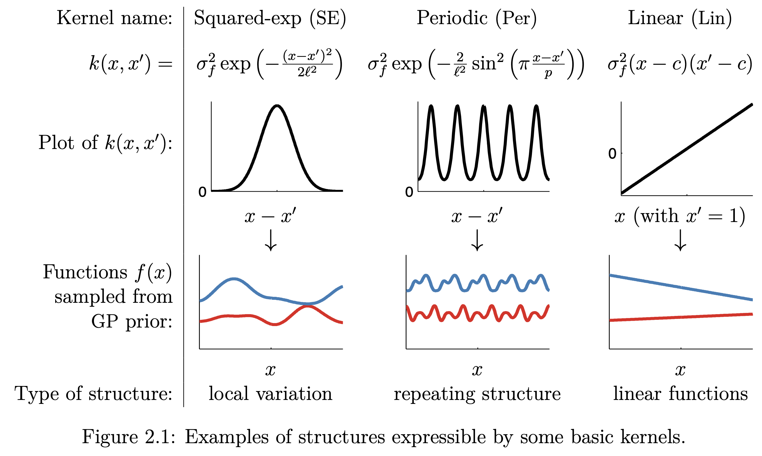
Fig. 7.2 Common GP kernels (Source: [Duvenaud, 2014]).#
Looking at a practical example of a possible kernel:
where \(\theta_{0}\), \(\theta_{1}\), \(\theta_{2}\), \(\theta_{3}\) are model hyperparameters. With the above \(p(y|x)\), we have identified which Gaussian is inferred from the data. Moreover, we have not yet formulated a predictive posterior for unseen data. For this purpose, we extend the data set
We reformulate the prediction problem as that of determining a conditional PDF. Given
we search for the conditional PDF \(p(y^{(n+1)}| y)\). As intermediate, we need the joint PDF
We assume that it also follows a Gaussian PDF. However, as \(x^{(n+1)}\) is unknown before prediction we have to make the dependence of the covariance matrix of \(p(\tilde{y})\) explicit. We first decompose the full covariance matrix into
with the vector
I.e. the corresponding entries in the extended \(\tilde{K} = \frac{1}{\alpha} \tilde{\Phi} \tilde{\Phi}^{\top}\) i.e. \(\tilde{K}_{1, \ldots, n+1}\), where \(\tilde{\Phi}_{n+1} = \varphi(x^{n+1})\). The \(c\)-entry above is then given by
Using the same approach as before, we can then calculate the mean and covariance of the predictive posterior for unseen data \(p(y^{(n+1)}|y)\). Recalling from before (Eq. (7.14)):
where we now adjust the entries for our present case with
And for the covariance \(\Sigma\) we recall
adjusting for the entries in our present case
From which follows
which fully defines the Gaussian posterior PDF of Gaussian-process regression.
Example: 1D GP with 1 measurement
Given is a single measurement data point \((x,y)=(1,2)\) with \(x,y\in \mathbb{R}\). Find \(p(y | x=1.25)\).
Solution: We start with our model assumption being fully described by the choice of noise variance \(\frac{1}{\beta}=10^{-6}\) and the kernel given by
We then substitute our values into equations (7.46) to obtain (up to three significant digits):
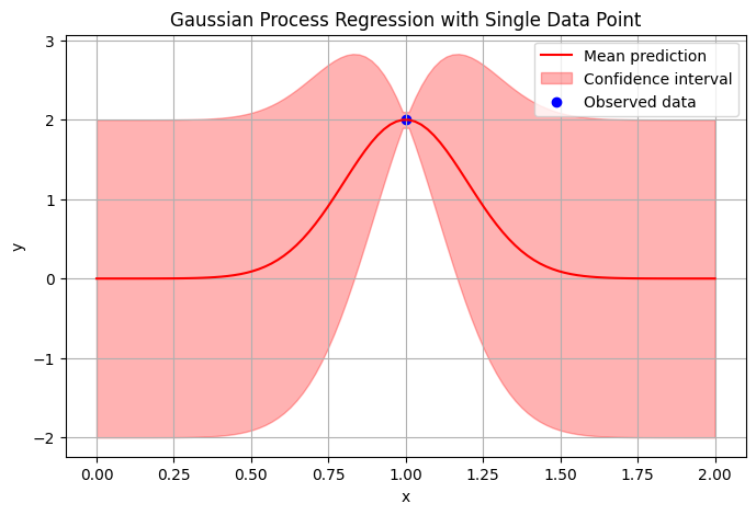
Fig. 7.3 GP example with confidence interval \(\pm 2\sigma\).#
Below we look at some sketches of GP regression, beginning with the data sample \(y_{1}\), and predicting the data \(y_{2}\)
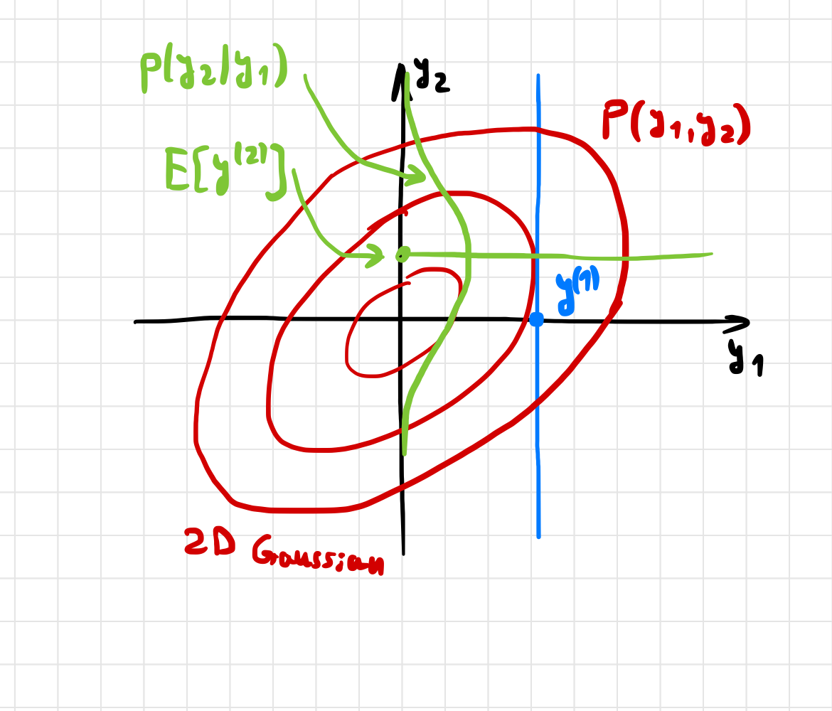
Fig. 7.4 Marginalizing a 2D Gaussian distribution.#
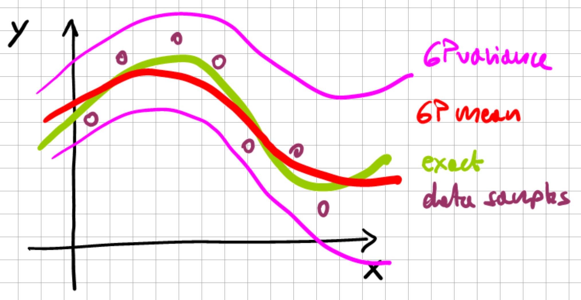
Fig. 7.5 1D Gaussian process.#
In practice, for a 1-dimensional function, which is being approximated with a GP, we monitor the change in the mean, variance, and synonymously the GP behavior (recall, the GP is defined by the behavior of its mean and covariance) with each successive data point.
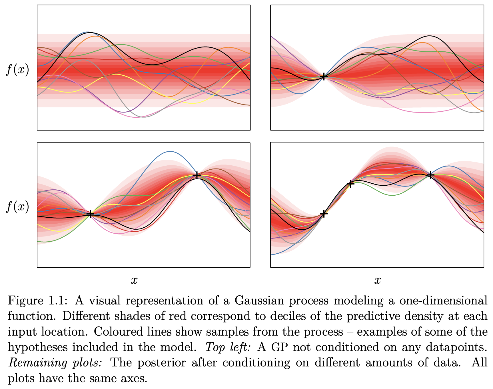
Fig. 7.6 Probability distribution of a 1D Gaussian process (Source: [Duvenaud, 2014]).#
This immediately shows the utility of GP-regression for engineering applications where we often have few data points but yet need to be able to provide guarantees for our predictions which GPs offer at a reasonable computational cost.
7.3.1. Further Kernel Configurations#
There exist many ways in which we can extend beyond just individual kernels by multiplication and addition of simple “basis” kernels to construct better-informed kernels. Just taking a quick glance at some of these possible combinations, where the following explores this combinatorial space for the following three kernels (see Fig. 7.2 for definitions):
Squared Exponential (SE) kernel
Linear (Lin) kernel
Periodic (Per) kernel
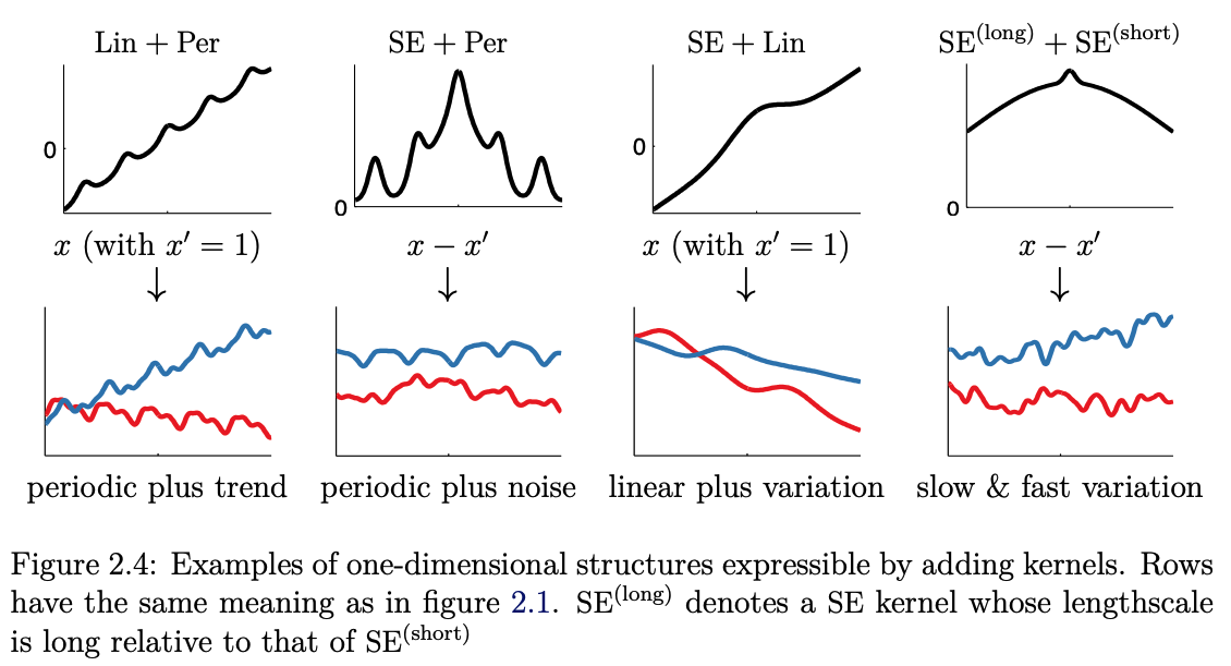
Fig. 7.7 Adding 1D kernels (Source: [Duvenaud, 2014]).#
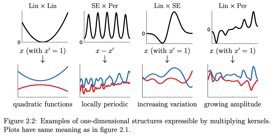
Fig. 7.8 Multiplying 1D kernels (Source: [Duvenaud, 2014]).#
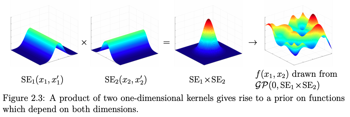
Fig. 7.9 Multiplying 1D kernels, 2D visualization (Source: [Duvenaud, 2014]).#
In higher dimensions, this then takes the following shape:
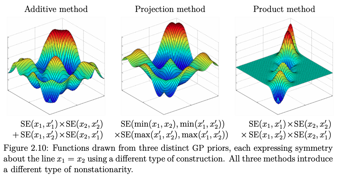
Fig. 7.10 Examples of 2D kernels (Source: [Duvenaud, 2014]).#
With all these possible combinations, one almost begs the question if these kernels cannot be constructed automatically. The answer is partially yes and partially no. In a sense, the right kernel construction is almost like feature engineering, and while it can be automated in parts, it remains a craft for the domain scientists to understand the nature of their problem to then construct the right prior distribution.
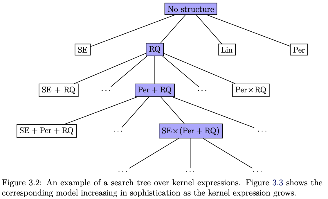
Fig. 7.11 Search tree over kernels (Source: [Duvenaud, 2014]).#
7.3.2. Multivariate Prediction#
The extension to multivariate prediction is then straightforward. For the unseen data
and for the sample data
for ever larger \(l\)’s the process can then just be repeated. The mean and covariance matrix are then given by
7.3.3. Notes on Gaussian Process Regression#
\(K + \frac{1}{\beta}I\) needs to be symmetric and positive definite, where positive definite implies that the matrix is symmetric. \(K\) can be constructed from valid kernel functions involving some hyperparameters \(\theta\).
GP regression involves a \(n \times n\) matrix inversion, which requires \(\mathcal{O}(n^{3})\) operations for learning.
GP prediction involves a \(n \times n\) matrix multiplication which requires \(\mathcal{O}(n^{2})\) operations.
The operation count can be reduced significantly when lower-dimensional projections of the kernel function on basis functions can be employed, or we are able to exploit sparse matrix computations.
7.3.4. Learning the Hyperparameters#
To infer the kernel hyperparameters from data, we need to:
Introduce an appropriate likelihood function \(p(y | \theta)\)
Determine the optimum \(\theta\) via maximum likelihood estimation (MLE) \(\theta^{\star} = \arg \max \ln p(y | \theta)\), which corresponds to linear regression
\(\ln p(y|\theta) = -\frac{1}{2} \ln |K + \frac{1}{\beta}I| - \frac{1}{2} y^{\top} \left( K + \frac{1}{\beta}I \right)^{-1} y - \frac{n}{2} \ln 2 \pi\)
Use iterative gradient descent or Newton’s method to find the optimum, where you need to be aware of the fact that \(p(y | \theta)\) may be non-convex in \(\theta\), and hence have multiple maxima
7.4. GP for Classification#
Without discussing all the details, we will now briefly sketch how Gaussian Processes can be adapted to classification. Consider for simplicity the 2-class problem:
The PDF for \(y\) conditioned on the feature \(\varphi(x)\) then follows a Bernoulli-distribution:
Finding the predictive PDF for unseen data \(p(y^{(n+1)}|y)\), given the training data
we then introduce a GP prior on
hence giving us
where \(K_{ij} = k(x^{(i)}, x^{(j)})\), i.e., a Grammian matrix generated by the kernel functions from the feature map \(\varphi(x)\).
Note that we do NOT include an explicit noise term in the data covariance as we assume that all sample data have been correctly classified.
For numerical reasons, we introduce a noise-like form \(\nu I\) that improves the conditioning of \(K\)
For two-class classification it is sufficient to predict \(p(y^{(n+1)} = 1 | y)\) as \(p(y^{(n+1)} = 0 | y) = 1 - p(y^{(n+1)} = 1 | y)\)
Using the PDF \(p(y=1|\varphi) = \text{sigmoid}(\varphi(x))\) we obtain the predictive PDF:
The integration of this PDF is analytically intractable, we are hence faced with a number of choices to integrate the PDF:
Use sampling-based methods, and Monte-Carlo approximation for the integral
Assume a Gaussian approximation for the posterior and evaluate the resulting convolution with the sigmoid in an approximating fashion
\(p(\varphi^{(n+1)}|y)\) is the posterior PDF, which is computed from the conditional PDF \(p(y| \varphi)\) with a Gaussian prior \(p(\varphi)\).
7.5. Relation of GP to Neural Networks#
We have not presented a definition of a neural network yet, but we have already met the most primitive definition of a neural network, the perceptron, for classification. The perceptron can be considered a neural network with just one layer of “neurons”. On the other hand, the number of hidden units should be limited for perceptrons to limit overfitting. The essential power of neural networks, i.e., the outputs sharing the hidden units, tends to get lost when the number of hidden units becomes very large. This is the core connection between neural networks and GPs, a neural network with infinite width recovers a Gaussian process.
7.6. Further References#
The Gaussian Distribution
[Bishop, 2006], Section 2.3
Gaussian Processes
[Bishop, 2006], Section 6.4
[Duvenaud, 2014], up to page 22
[Rasmussen and Williams, 2006], Sections 2.1-2.6