4. Optimization

In the lecture on Linear Models, we already saw the main building blocks of a supervised learning algorithm:

1. Model \(h\) of the relationship between inputs \(x\) and outputs \(y\),

2. Loss (aka Cost, Error) function \(J(\vartheta)\) quantifying the discrepancy between \(h_{\vartheta}(x^{(i)})\) and \(y^{(i)}\) for each of the measurement pairs \(\left\{(x^{(i)}, y^{\text {(i)}})\right\}_{i=1,...m}\), and

3. Optimization algorithm (aka Optimizer) minimizing the loss.

Point 1 is a matter of what we know about the world in advance and how we include that knowledge into the model, e.g. choose CNNs when working with images because the same pattern might appear at different locations of an image. Later in the lecture, we will look at different models each of which is by construction better suited for different problem types.

After selecting a model \(h_{\vartheta}\), points 2 and 3 are critical to the success of the learning as the loss function (point 2) defines how we measure success and the optimizer (point 3) guides the process of moving from a random initial guess of the parameters to a parameter configuration with a smaller loss. These two points are the topic of this lecture and the lecture Tricks of Optimization.

Note: all algorithms discussed below assume an unconstrained parameter space, i.e. \(\vartheta \in \mathbb{R}^n\). There are dedicated algorithms for solving constraint optimization problems, e.g. \(a \le \vartheta \le b\), but these are beyond the scope of our lecture.

4.1. Basics of Optimization

First, we define the general (unconstrained) minimization problem

(4.1)\[\text{argmin}_{\vartheta} \; J(\vartheta),\]

where \(J:\mathbb{R}^n \rightarrow \mathbb{R}\) is a real-valued function. We call the optimal solution of this problem the minimizer of \(J\) and denote it as \(\vartheta_{\star}\). The minimizer is defined as \(J(\vartheta_{\star}) \le J(\vartheta)\) for all \(\vartheta\). If the relation \(J(\vartheta_{\star}) \le J(\vartheta)\) holds only in a local neighborhood \(||\vartheta - \vartheta_{\star}|| \le \epsilon\), for some \(\epsilon>0\), then we call \(\vartheta_{\star}\) a local optimizer.

In the figure below we an example of different loss functions.

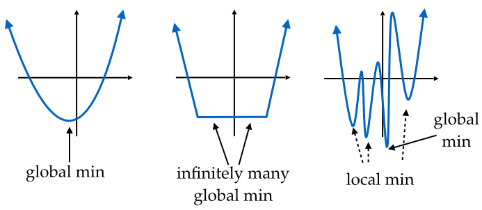
Fig. 4.1 Function with (left) one global minimum, (middle) infinitely many global minima, and (right) multiple local as well as one global minimum (Source: [Hardt and Recht, 2022], Chapter 5).

4.1.1. Convexity

Convexity is a property of a function and has a simple geometric meaning.

If the function \(J\) fulfills the following inequality

(4.2)\[J(\alpha \vartheta_l+(1-\alpha)\vartheta_r) \le \alpha J(\vartheta_l)+(1-\alpha)J(\vartheta_r), \quad \forall \vartheta_l, \vartheta_r \text{ and } \alpha \in [0,1],\]

then \(J\) is said to be convex. Geometrically, this inequality implies that a line segment between \((\vartheta_l, J(\vartheta_l))\) and \((\vartheta_r, J(\vartheta_r))\) lies above the graph of \(J\) in the range \((\vartheta_l, \vartheta_r)\).

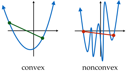
Fig. 4.2 Example of convex and nonconvex function (Source: [Hardt and Recht, 2022], Chapter 5).

There is exhaustive literature on convex functions and convex optimization, e.g. [Boyd and Vandenberghe, 2004], due to the mathematical properties of such functions. An important result from this theory is that gradient descent is guaranteed to find an optimum of a convex function.

Two examples of convex functions are the Least Mean Square loss in linear regression and the negative log-likelihood in logistic regression. However, modern deep learning is in general non-convex. Thus, we optimize towards a local minimum in the proximity of an initial configuration.

Note: Convexity is a property of the loss \(J(\vartheta)\) w.r.t. \(\vartheta\). This means, for \(J(\vartheta)\) to be convex, the combination of model and loss functions has to result in a convex function in \(\vartheta\).

Apparently, the choice of \(h(x)\) plays an important role in the shape of \(J(\vartheta)\), but how does the choice of loss function influence \(J\)?

4.1.2. Cost Functions

We will discuss extensions of the loss function in the lecture Tricks of Optimization. For now, we give an example of common loss functions by problem type:

• Regression loss

  • L1 loss: \(\; \; \; J(h_{\vartheta}(x), y)=1/m \sum_{i=1}^m |y-h_{\vartheta}(x)|\)

  • MSE loss: \(J(h_{\vartheta}(x), y)=1/m \sum_{i=1}^m (y-h_{\vartheta}(x))^2\)

• Classification loss

  • Cross Entropy loss \(J(h_{\vartheta}(x),y)= -\sum_{i=1}^m\sum_{k=1}^K(y_{ik}\cdot \log h_{\vartheta, k}(x_i))\)

4.2. Gradient-based Methods

If we now consider the functions from Fig. 4.1 as highly simplified objective functions which we want to minimize, then we see that the gradient descent method we saw in lecture Linear Models is well suited. While being the obvious choice for the two cases on the left, the picture becomes a little muddier in the example on the right.

Notation alert: For the derivation of the gradien-based optimization techniques we use the stands notation by which the function we want to find the minimum of becomes \(J \rightarrow f\) and the variable \(\vartheta \rightarrow x\). Don’t confuse this \(x\) with the input measurements \(\{x^{(i)},y^{(i)}\}_{i=0,...,m}\).

4.2.1. Gradient Descent

While the foundational concept, gradient descent is rarely used in its pure form, but mostly in its stochastic form these days. If we first consider it in its most foundational form in 1-dimension, then we can take a function \(f\), and Taylor-expand it

(4.3)\[f(x+\varepsilon) = f(x) + \varepsilon f'(x) + \mathcal{O}(\varepsilon^{2}).\]

Then, our intuition would dictate that moving a small \(\varepsilon\) in the direction of the negative gradient will decrease f. Taking a step size \(\eta > 0\), and using using our ability to freely choose \(\varepsilon\) to set it as

(4.4)\[\varepsilon = - \eta f'(x),\]

to then be plugged back into the Taylor expansion leads to

(4.5)\[f(x - \eta f'(x)) = f(x) - \eta f'^{2}(x) + \mathcal{O}(\eta^{2}f'^{2}(x)).\]

Unless our gradient vanishes, we can then minimize \(f\) as \(\eta f'^{2}(x)>0\). Choosing a small enough \(\eta\) can then make the higher-order terms irrelevant to arrive at

(4.6)\[f(x - \eta f'(x)) \leq f(x)\]

I.e.

(4.7)\[x \leftarrow x - \eta f'(x)\]

is the right algorithm to iterate over \(x\) s.t. the value of our (objective) function \(f(x)\) declines. We hence end up with an algorithm in which we have to choose an initial value for \(x\), a constant \(\eta > 0\), and then continuously iterate \(x\) until we reach our stopping criterion.

\(\eta\) is most commonly known as our learning rate and has to be set by us. Now, if \(\eta\) is too small \(x\) will update too slowly and require us to perform many more costly iterations than we’d ideally like to. But if we choose a learning rate that is too large, then the error term \(\mathcal{O}(\eta^{2}f'^{2}(x))\) at the back of the Taylor-expansion will explode, and we will overshoot the minimum.

Now, if we take a non-convex function for \(f\) which might even have infinitely many local minima, then the choice of our learning rate and initialization becomes even more important. Take the following function \(f\) for example:

(4.8)\[f(x) = x \cdot \cos(cx).\]

Then the optimization problem might end up looking like the following:

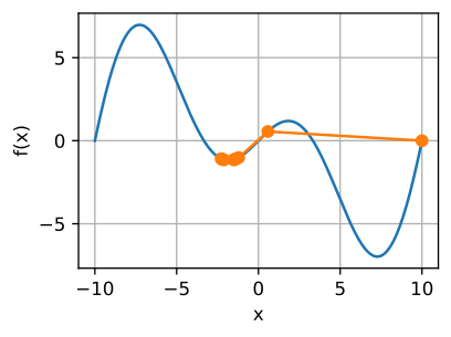
Fig. 4.3 Optimizing \(f(x) = x \cdot \cos(cx)\) (Source: [Zhang et al., 2021], here).

\(x\) as vector

If we now consider the case where we do not only have a one-dimensional function \(f\), but instead a function s.t.

(4.9)\[f: \mathbb{R}^{d} \rightarrow \mathbb{R},\]

i.e. a vector is mapped to a scalar, then the gradient is a vector of \(d\) partial derivatives

(4.10)\[\nabla f({\bf{x}}) = \left[ \frac{\partial f({\bf{x}})}{\partial x_{1}}, \frac{\partial f({\bf{x}})}{\partial x_{2}}, \ldots, \frac{\partial f({\bf{x}})}{\partial x_{d}} \right]^{\top},\]

with each term indicating the rate of change in each of the \(d\) dimensions. Then, we can use the Taylor-approximation as before and derive the gradient descent algorithm for the multivariate case

(4.11)\[{\bf{x}} \leftarrow {\bf{x}} - \eta \nabla f({\bf{x}})\]

If we then construct an objective function such as

(4.12)\[f({\bf{x}}) = x_{1}^{2} + 2 x_{2}^{2},\]

then our optimization could take the following shape.

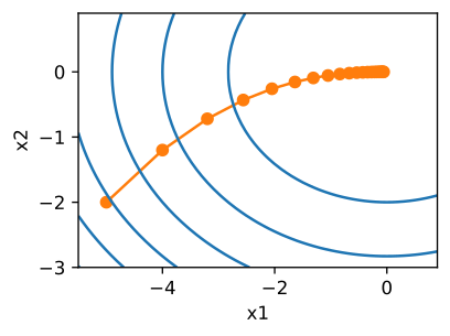
Fig. 4.4 Optimizing \(f({\bf{x}}) = x_{1}^{2} + 2 x_{2}^{2}\) (Source: [Zhang et al., 2021], here).

Having up until now relied on a fixed learning rate \(\eta\), we now want to expand upon the previous algorithm by adaptively choosing \(\eta\). For this, we have to go back to Newton’s method.

For this, we have to further expand the initial Taylor-expansion to the third-order term

(4.13)\[f({\bf{x}} + {\bf{\varepsilon}}) = f({\bf{x}}) + {\bf{\varepsilon}}^{\top} \nabla f({\bf{x}}) + \frac{1}{2} {\bf{\varepsilon}}^{\top} \nabla^{2} f({\bf{x}}) {\bf{\varepsilon}} + \mathcal{O}(||{\bf{\varepsilon}}||^{3}).\]

If we now look closer at \(\nabla^{2} f({\bf{x}})\), sometimes also called the Hessian, then we recognize that for larger problems this term might be infeasible to compute due to the required \(\mathcal{O}(d^{2})\) computations.

Following the condition \(\nabla_{\epsilon} f(\bf{x} + \epsilon)=0\) for the minimum to calculate \(\varepsilon\), we then arrive at the ideal value of

(4.14)\[{\bf{\varepsilon}} = - (\nabla^{2} f({\bf{x}}))^{-1} \nabla f({\bf{x}})\]

I.e. we need to invert \(\nabla^{2} f({\bf{x}})\), the Hessian. Computing and storing this important array turns out to be really expensive! To reduce these costs we are looking towards the preconditioning of our optimization algorithm. For preconditioning we then only need to compute the diagonal entries, hence leading to the following update equation

(4.15)\[{\bf{x}} \leftarrow {\bf{x}} - \eta \text{diag }(\nabla^{2} f({\bf{x}}))^{-1} \nabla f({\bf{x}}).\]

What the preconditioning then achieves is to select a specific learning rate for every single variable.

4.2.1.1. Momentum

If we now have a mismatch in the scales of two variables contained in our objective function, then we end up with an unsolvable optimization problem. To solve it, we require the momentum method

(4.16)\[\begin{split} \begin{aligned} {\bf{v}}_{t} &\leftarrow \beta {\bf{v}}_{t-1} + {\bf{g}}_{t} \\ {\bf{x}}_{t} &\leftarrow {\bf{x}}_{t-1} - \eta_{t} {\bf{v}}_{t}, \end{aligned} \end{split}\]

with gradients of the loss \(\mathbf{g}_t = \nabla f_t(x)\) and the momentum variable \(\mathbf{v}_t\). The momentum \(\mathbf{v}_t\) accumulates past gradients resembling how a ball rolling down a hill integrates over past forces. For \(\beta=0\), we then have the regular gradient descent update. To now choose the perfect effective sample weight, we have to take the limit of

(4.17)\[{\bf{v}}_{t}\ = \sum_{\tau = 0}^{t-1} \beta^{\tau} {\bf{g}}_{t-\tau}.\]

Taking the limit \(t \to \infty\) results in the geometric series solution

(4.18)\[\sum_{\tau=0}^{\infty} \beta^{\tau} = \frac{1}{1 - \beta}\]

Hence using the momentum GD results in a step size \(\frac{\eta}{1 - \beta}\), which at the same time gives us much better gradient descent directions to follow to minimize our objective function.

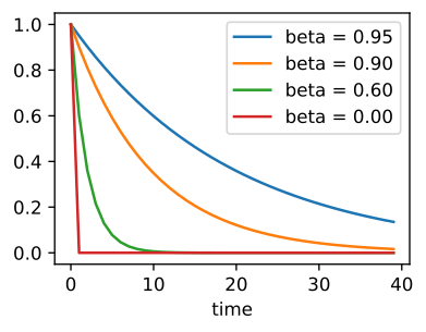
Fig. 4.5 Momentum parameter (Source: [Zhang et al., 2021], here).

4.2.2. Adam

The Adam algorithm, then extends beyond traditional gradient descent by combining multiple tricks into a highly robust algorithm, which is one of the most often used optimization algorithms in machine learning.

Expanding upon the previous use of momentum, Adam further utilizes the 1st and 2nd momentum of the gradient, i.e.

(4.19)\[\begin{split} \begin{aligned} {\bf{v}}_{t} &\leftarrow \beta_{1} {\bf{v}}_{t-1} + (1 - \beta_{1}) {\bf{g}}_{t} \\ {\bf{s}}_{t} &\leftarrow \beta_{2} {\bf{s}}_{t-1} + (1 - \beta_{2}) {\bf{g}}_{t}^{2}, \end{aligned} \end{split}\]

where both \(\beta_{1}\), and \(\beta_{2}\) are non-negative. A typical initialization here would be something along the lines of \(\beta_{1} = 0.9\), and \(\beta_{2} = 0.999\) s.t. the variance estimate moves much slower than the momentum term. As an initialization of \({\bf{v}}_{0} = {\bf{s}}_{0} = 0\) can lead to bias in the optimization algorithm towards small initial values, we have to re-normalize the state variables with

(4.20)\[{\hat{\bf{v}}}_{t} = \frac{{\bf{v}}_{t}}{1 - \beta_{1}^{t}} \text{, and } {\hat{\bf{s}}}_{t} = \frac{{\bf{s}}_{t}}{1 - \beta_{2}^{t}}.\]

The Adam optimization algorithm then rescales the gradient to obtain

(4.21)\[{\bf{g}}'_{t} = \frac{\eta {\hat{\bf{v}}}_{t}}{\sqrt{{\hat{\bf{s}}}_{t}} + \varepsilon}.\]

The update formula for Adam is then

(4.22)\[{\bf{x}}_{t} \leftarrow {\bf{x}}_{t-1} - {\bf{g}}'_{t}.\]

The strength of the Adam optimization algorithm is the stability of its update rule.

If the momentum GD algorithm can be understood as a ball rolling down a hill, the Adam algorithm behaves like a ball with friction (see GANs Trained by a Two Time-Scale Update Rule Converge to a Local Nash Equilibrium).

Fig. 4.6 Comparison of 1st order optimization algorithms (Source: github.com/Jaewan-Yun/optimizer-visualization).

4.2.3. Stochastic Gradient Descent

In machine learning, we could take the loss across an average of the entire training set. Writing down the objective function for the training set with \(n\) entries leads to

(4.23)\[f({\bf{x}}) = \frac{1}{n} \sum_{i=1}^{n}f_{i}({\bf{x}}).\]

Here, \(f_i\) refers to evaluating the loss for training sample \(i\), and \(\bf{x}\) denotes the model parameter vector. The gradient of the objective function is then

(4.24)\[\nabla f({\bf{x}}) = \frac{1}{n} \sum_{i=1}^{n} \nabla f_{i}({\bf{x}}).\]

With the cost of each independent variable iteration being \(\mathcal{O}(n)\) for gradient descent, stochastic gradient replaces this with a sampling step where we uniformly sample an index \(i \in \{1, \ldots, n\}\) at random, and then compute the gradient for the sampled index, and update \({\bf{x}}\)

(4.25)\[{\bf{x}} \leftarrow {\bf{x}} - \eta \nabla f_{i}({\bf{x}}).\]

With this randomly sampled update, the cost for each iteration drops to \(\mathcal{O}(1)\). Due to the sampling we now have to think of our gradient as an expectation, i.e. by drawing uniform random samples we are essentially creating an unbiased estimator of the gradient

(4.26)\[\mathbb{E}_{i} \nabla f_{i}({\bf{x}}) = \frac{1}{n} \sum_{i=1}^{n} \nabla f_{i}({\bf{x}}) = \nabla f({\bf{x}})\]

Looking at an example stochastic gradient descent optimization process in Fig. 4.7, we come to realize that the stochasticity induces too much noise for our chosen learning rate. To handle that we later introduce learning rate scheduling.

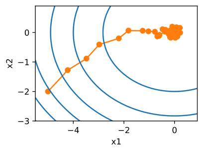
Fig. 4.7 SGD trajectory (Source: [Zhang et al., 2021], here).

4.2.3.1. Minibatching

For data which is very similar, gradient descent is inefficient, whereas stochastic gradient descent relies on the power of vectorization.

The answer to these ailments is the use of minibatches to exploit the memory and cache hierarchy a modern computer exposes to us. In essence, we seek to avoid the many single matrix-vector multiplications to reduce the overhead and improve our computational cost. If we compute the gradient in stochastic gradient descent as

(4.27)\[{\bf{g}}_t = \nabla f({\bf{x}}, i),\]

then, for computational efficiency, we will now perform this update in its batched form

(4.28)\[{\bf{g}}_t = \nabla \frac{1}{|\mathcal{B}_{t}|} \sum_{i \in \mathcal{B}_{t}} f({\bf{x}}, i).\]

As both \(\bf{g}_t\) and \(i\) are drawn uniformly at random from the training set, we retain our unbiased gradient estimator. For size \(b\) of the dataset, i.e \(b = | \mathcal{B}_{t} |\) we obtain a reduction of the standard deviation by \(b^{-\frac{1}{2}}\), while this is desirable we should in practice choose the minibatch-size s.t. our underlying hardware gets utilized as optimally as possible.

4.3. Second-Order Methods

With first-order methods only taking the gradient itself into account there is much information we are leaving untapped in attempting to solve our optimization problem, such as gradient curvature for which we’d need 2nd order gradients.

The reason for that is in part historic, automatic differentiation (to be explained in-depth in a later lecture) suffers from an exponential compute-graph blow-up when computing higher-order gradients. The automatic differentiation engines, the first popularized machine learning engines from AlexNet, LeNet etc. were built on, were unable to handle higher-order gradients for the above reason, and only modern automatic differentiation engines have been able to circumvent that problem. As such 2nd-order gradient methods have seen a recent resurgence with methods like Shampoo, RePAST, and Fishy.

4.3.1. Newton’s method

(also Newton-Raphson method)

A first example of the step toward second-order methods is the Newton method. It is an iterative method to find a zero of a differentiable function defined as \(f: \mathbb{R} \rightarrow \mathbb{R}\). The Newton-method begins with an initial guess \(x_{0}\) to then iteratively update with

(4.29)\[x_{t+1} = x_{t} - \frac{f(x_{t})}{f'(x_{t})}\]

Graphically speaking this amounts to the case of the tangent line of the function intersecting with the x-axis.

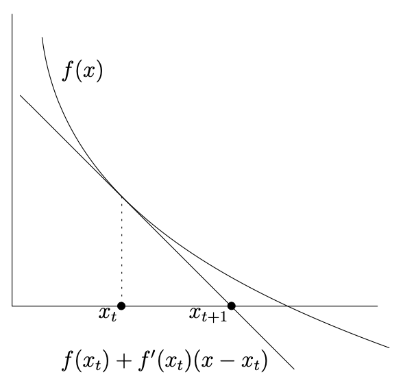
Fig. 4.8 Newton’s method (Source: [Gärtner and Jaggi, 2023], Chapter 7).

The fallacies of this method are the cases where \(f'(x_{t}) = 0\), and it will diverge when \(|f'(x_{t})|\) is very small. Going beyond the first-order update, we can then utilize the second-order gradient if our (objective) function \(f\) is twice differentiable. Hence turning the update step into

(4.30)\[x_{t+1} = x_{t} - \frac{f'(x_{t})}{f''(x_{t})}, \quad t>0\]

Generalizing this update scheme in notation, we can use vector calculus to obtain

(4.31)\[x_{t+1} = x_{t} - \nabla^{2} f(x_{t})^{-1} \nabla f(x_{t}), \quad t\geq 0\]

\(\nabla^{2} f(x_{t})^{-1}\) constitutes the inverse of the Hessian at \(x_{t}\). As alluded to earlier the failure modes can then be formalized in the following fashion:

• The Hessian is not invertible.

• Gets out of control if the Hessian has a small norm.

If we further generalize the notation to a general update scheme

(4.32)\[x_{t+1} = x_{t} - \tilde{H}(x_{t}) \nabla f(x_{t})\]

then we can simplify this update scheme to the gradient descent we already encountered in the last lecture by setting \(\tilde{H}(x_{t}) = \gamma I\), where \(I\) is the identity matrix. With \(\tilde{H}=\nabla^2f(x)^{-1}\) we recover Newton’s method. Newton’s method hence constitutes an adaptive gradient descent approach, where the adaptation happens with respect to the local geometry of the objective function at \(x_{t}\).

Where gradient descent requires the right step-size, Newton’s method converges naturally to the local minimum without the requirement of step-size tuning.

To expand upon this, assume we have a linear system of equations

(4.33)\[M {\bf{x}} = {\bf{q}},\]

then Newton’s method can solve this system in one step whereas gradient descent requires multiple steps with the right step size chosen. The downside to this is the expensive step of inverting matrix \(M\). In our general case, this means we need to invert the expensive matrix \(\nabla^{2} f(x_{0})\).

Another advantage of Newton’s method is that it does not suffer from individual coordinates being at completely different scales, e.g. the \(y\)-direction changes very fast, whereas the \(z\)-direction only changes very slowly. Gradient descent only handles these cases suboptimally, whereas Newton’s method does not suffer from this shortcoming.

Note: The Hessian has to be positive definite, otherwise we would end up in a local maximum.

A matrix \(H\) is positive definite if the real number \(z^{\top} H z\) is positive for every nonzero real-valued vector \(z\).

4.3.2. The Quasi-Newton Approach

With the main computational bottleneck of Newton’s approach being that the inversion of the Hessian matrix costs \(\mathcal{O}(d^{3})\) for a matrix of size \(d \times d\), there exist multiple approaches which try to circumvent this costly operation.

4.3.2.1. The Secant Method

The secant method is an alternative to Newton’s method, which consciously does not use derivatives and has hence much less stringent requirements on our objective function such as it not needing to be differentiable. We can replace the derivative in Newton’s method with the finite difference approximation, i.e.

(4.34)\[\frac{f(x_{t}) - f(x_{t-1})}{x_{t} - x_{t-1}} \approx f'(x_{t})\]

for a small region around \(x_{t}\). The secant update step then takes the following form

(4.35)\[x_{t+1} = x_{t} - f(x_{t})\frac{x_{t} - x_{t-1}}{f(x_{t}) - f(x_{t-1})}, \quad t\geq 1\]

to approximate the Newton step at the detriment of having to choose two starting values \(x_{0}\), and \(x_{1}\) here. Figuratively speaking, the approach looks like this:

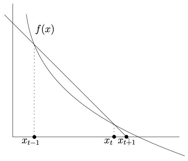
Fig. 4.9 Secant method (Source: [Gärtner and Jaggi, 2023], Chapter 8).

What this approach then does is to construct the line through the two points \((x_{t-1}, f(x_{t-1}))\), and \((x_{t}, f(x_{t}))\) on the graph of f, the next iteration is then given by the point where the line intersects the x-axis.

When our function is first-order differentiable, we can also use the secant method to derive a second-derivative-free version of Newton’s method for optimization.

(4.36)\[x_{t+1}=x_{t} - f'(x_{t})\frac{x_{t} - x_{t-1}}{f'(x_{t}) - f'(x_{t-1})}, \quad t \geq 1.\]

4.3.2.2. Quasi-Newton Methods

If we consider the so-called secant condition, then we have the following approximation

(4.37)\[H_{t} = \frac{f'(x_{t}) - f'(x_{t-1})}{x_{t} - x_{t-1}} \approx f''(x_{t}),\]

then the secant method works with the following update step using the above approximation

(4.38)\[x_{t+1} = x_{t} - H_{t}^{-1}f'(x_{t}), \quad t \geq 1.\]

For this approximation to hold we need to satisfy the secant condition

(4.39)\[f'(x_{t}) - f'(x_{t-1}) = H_{t}(x_{t} - x_{t-1}).\]

Or generalized to higher dimensions

(4.40)\[\nabla f({\bf{x_{t}}}) - \nabla f({\bf{x_{t-1}}}) = H_{t}({\bf{x_{t}}} - {\bf{x_{t-1}}}).\]

Whenever this condition is now fulfilled in conjunction with a symmetric matrix, then we have a Quasi-Newton method. As our matrix \(H_{t} \approx \nabla^{2}f(x_{t})\) only fluctuates very little during periods of very fast convergence, and Newton’s method is optimal with one step, then we can presume

(4.41)\[H_{t} \approx H_{t-1}\]

and equally as much

(4.42)\[H_{t}^{-1} \approx H_{t-1}^{-1},\]

then we can (following Greenstadt’s approach) model \(H_{t}\) in the following fashion

(4.43)\[H_{t}^{-1} = H^{-1}_{t-1} + E_{t}.\]

I.e. our matrix \(H_{t}\), the Hessian, only changes by a minor error matrix \(E_t\). These errors should also be as small as possible.

4.3.2.3. BFGS

(Broyden–Fletcher–Goldfarb–Shanno)

For the BFGS algorithm, this update matrix then assumes the form

(4.44)\[E = \frac{1}{{\bf{y}}^{\top} {\bf{\sigma}}} \left( -H {\bf{y}} {\bf{\sigma}}^{\top} - {\bf{\sigma}} {\bf{y}}^{\top} H + (1 + \frac{{\bf{y}}^{\top}H{\bf{y}}}{{\bf{y}}^{\top} {\bf{\sigma}}}) {\bf{\sigma}} {\bf{\sigma}}^{\top} \right),\]

where we simplified notation to \(H=H_{t-1}^{-1}\), \({\bf{\sigma}} = x_{t} - x_{t-1}\), and \(y = \nabla f(x_{t}) - \nabla f(x_{t-1})\).

One of the core advantages of BFGS is that if \(H':=H_{t}^{-1}\) is positive definite, then the update \(E\) maintains this positive definite attribute and as such behaves like a proper inverse Hessian. In addition, the cost of computation drops from the original \(\mathcal{O}(d^{3})\) for a matrix of size \(d \times d\) to \(\mathcal{O}(d^{2})\) for the BFGS approach. Scaling the update step, the individual iteration then becomes

(4.45)\[x_{t+1} = x_{t} - \alpha_{t} H_{t}^{-1} \nabla f(x_{t}), \quad t \geq 1\]

where \(\alpha\) can be chosen such that a line search is performed, and where \(H_{t}^{-1}\) is the BFGS approximation. In a pseudo-algorithmic form this then looks the following way:

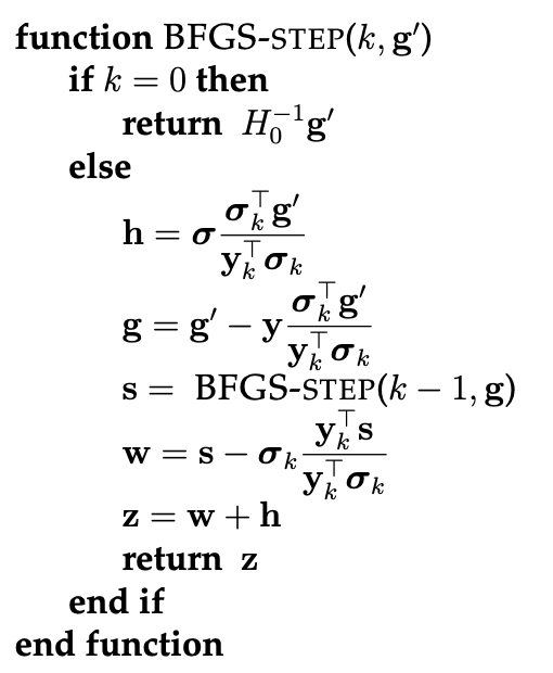
Fig. 4.10 BFGS algorithm (Source: [Gärtner and Jaggi, 2023], Chapter 8).

4.3.2.4. L-BFGS

(Limited-memory BFGS)

Especially in high dimensions a cost of \(\mathcal{O}(d^{2})\) may still be too prohibitive. Only using information from the past \(m\) iterations for \(m\) being a small value, L-BFGS then approximates the entire \(H'\nabla f(x_{t})\) term. L-BFGS then builds on modeling \(H'\) as

(4.46)\[H' = \left( I - \frac{\sigma y^{\top}}{y^{\top}\sigma} \right) H \left( I - \frac{y \sigma^{\top}}{y^{\top}\sigma} \right) + \frac{\sigma \sigma^{\top}}{y^{\top} \sigma}.\]

Then, we are able to utilize an oracle to compute

(4.47)\[s= H g\]

for any vector \(g\). Then \(s' = H'g'\) can be computed with one oracle call and \(\mathcal{O}(d)\) additional arithmetic operations, assuming that \(\sigma\), and \(y\) are known. We then define \(\sigma\), and \(y\) in the following fashion

(4.48)\[\begin{split}\begin{align} \sigma_{k} &= x_{k} - x_{k-1} \\ y_{k} &= \nabla f(x_{k}) - \nabla f(x_{k-1}) \end{align}\end{split}\]

The L-BFGS algorithm is then given by

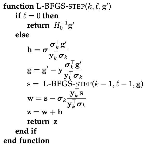
Fig. 4.11 L-BFGS algorithm (Source: [Gärtner and Jaggi, 2023], Chapter 8).

where in the case of the recursion bottoming out prematurely at a point \(k=t-m\), then we pretend that we just started the computation at that point and use \(H_{0}\).

4.4. Derivative-Free Optimization (DFO)

(also Blackbox optimizations)

If we are unable to compute gradients for any reason, then we need to rely on derivative-free optimization (DFO). This is most commonly used in blackbox function optimization, or discrete optimization.

If you as an engineer would have to optimize the design of some model given to you, but where you are not allowed to touch the code or even look at the code of the model, but only query it for outputs, then this would constitute a case of blackbox function optimization.

There exist a number of approaches for such problems, which all depend on the cost of evaluation of our function.

• Expensive function

  • Bayesian optimization

• Cheap function

  • Stochastic local search

  • Evolutionary search

In local search, for example, we replace the entire gradient update with

(4.49)\[x_{t+1} = \underset{x \in nbr(x_{t})}{\text{argmax}}\]

where \(nbr\) is the neighborhood of the point \(x_{t}\). This approach is also colloquially known as hill climbing, steepest ascent, or greedy search. In stochastic local search, we would then define a probability distribution over the uphill neighbors proportional to how much they improve our function and then sample at random. A second stochastic option is to start again from a different random starting point whenever we reach a local maximum. This approach is known as random restart hill climbing.

An effective strategy here is also random search, which should be the go-to baseline one attempts first when approaching a new problem. Here an iterate \(x_{t+1}\) is chosen uniformly at random from the set of iterates. An alternative, which has been proven to be less efficient (see Random Search for Hyper-Parameter Optimization by Bergstra and Bengio, 2012), is the grid search, which chooses hyperparameters equidistantly in the same range used for random search.

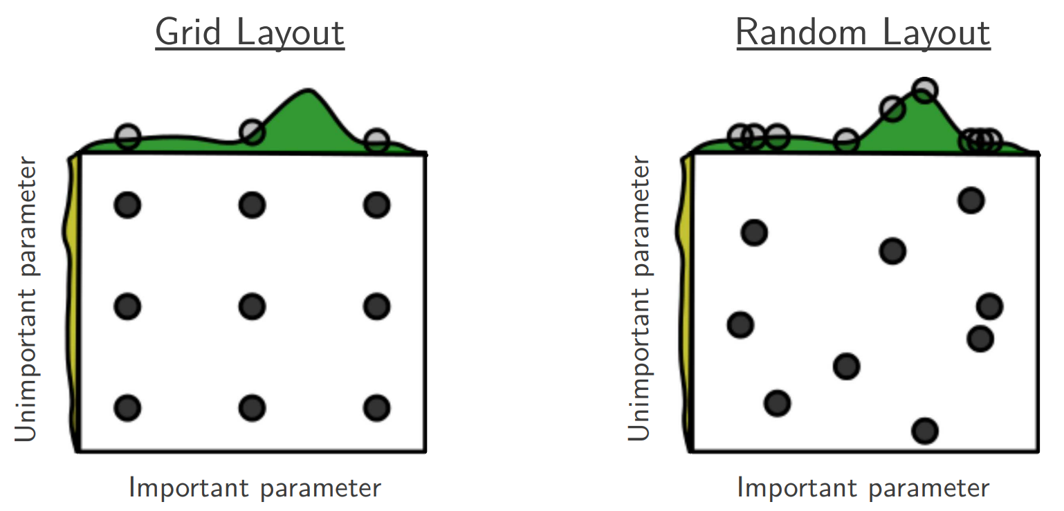
Fig. 4.12 Grid search vs random search (Source: Random Search for Hyper-Parameter Optimization).

If instead of throwing away our “old” good candidates keep them in a population of good candidates, then we arrive at evolutionary algorithms. Here we maintain a population of \(K\) good candidates, which we then try to improve at each step. The advantage here is that evolutionary algorithms are embarrassingly parallel and are as such highly scalable.

4.5. Further References

Basics of Optimization

• [Hardt and Recht, 2022], Chapter 5

• [Boyd and Vandenberghe, 2004], Chapter 1

First-Order Optimization

• [Hardt and Recht, 2022], Chapter 5

• [Zhang et al., 2021], Chapter Optimization Algorithms

• [Boyd and Vandenberghe, 2004], Chapter 9

• An overview of gradient descent optimization algorithms, S. Ruder, 2016

Second-Order Optimization

• [Gärtner and Jaggi, 2023], Chapters 7 and 8

• [Nocedal and Wright, 2006], Chapters 3 and 6