11. Recurrent Models#
Learning outcome
How to design a neural network that operates on sequences?
Which probabilistic model can be used to describe sequence generation/classification?
What are the weaknesses of simple RNNs, and how does the LSTM help?
While CNNs and MLPs are excellent neural network architectures for spatial relations, they yet struggle with the modeling of temporal relations which they are incapable of modeling in their default configuration. The figure below gives an overview of different task formulations.
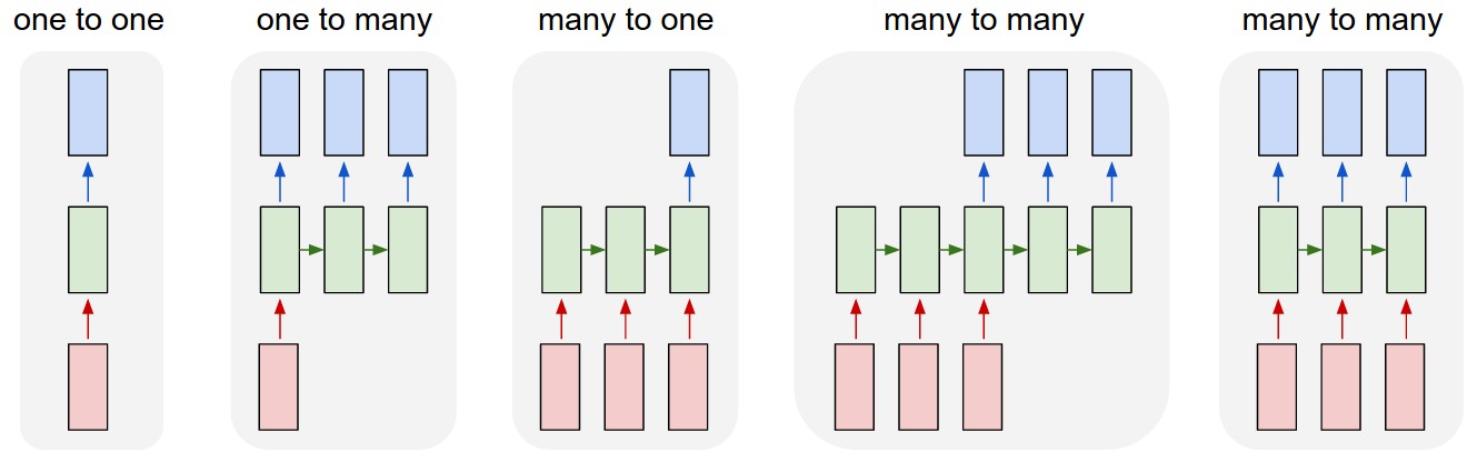
Fig. 11.1 Types of sequences (Source: karpathy.github.io)#
For such tasks, there exist a number of specialized architectures, most notably:
While Transformers have become the dominant architecture in machine learning these days, their roots lie in the development of RNNs, from whom we will begin to build up the content of this section to introduce the architectures in order, show their similarities, as well as special properties and where you most appropriately deploy them.
11.1. Recurrent Neural Networks (RNNs)#
While CNNs map from an input space of images, Recurrent Neural Networks (RNNs) map from an input space of sequences to an output space of sequences. RNN’s core property is the stateful prediction, i.e., if we seek to predict an output \(y\), then \(y\) depends not only on the input \(x\) but also on the hidden state of the system \(h\). The hidden state of the neural network is updated as time progresses during the processing of the sequence. There are a number of use cases for such models, such as:
Sequence Generation
Sequence Classification
Sequence Translation
We will be focussing on the three in the very same order.
11.1.1. Sequence Generation#
Sequence generation can mathematically be summarized as
with an input vector of size \(D\), and an output sequence of \(N_{\infty}\) vectors each with size \(C\). As we are essentially mapping a vector to a sequence, these models are also called vec2seq models. The output sequence is generated one token at a time, where we sample at each step from the current hidden state \(h_{t}\) of our neural network, which is subsequently fed back into the model to update the hidden state to the new state \(h_{t+1}\).
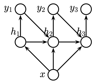
Fig. 11.2 Vector to sequence task (Source: [Murphy, 2022], Chapter 15)#
To summarize, a vec2seq model is a probabilistic model of the form \(p(y_{1:T}|x)\). If we now break this probabilistic model down into its actual mechanics, then we end up with the following conditional generative model
Just like a Runge-Kutta scheme, this model requires seeding with an initial hidden state distribution. This distribution has to be predetermined and is most often deterministic. The computation of the hidden state is then presumed to be
for the deterministic function \(f\). A typical choice constitutes
with \(W_{hh}\) the hidden-to-hidden weights, and \(W_{xh}\) the input-to-hidden weights. The output distribution is then either given by
where “Cat” is the categorical distribution in the case of a discrete output from a predefined set, or by something like
for real-valued outputs. Now if we seek to express this in code, then our model looks something like this:
def rnn(inputs, state, params):
    # Referring to Karpathy's drawing above, we present the right-most case many-to-many
    # Here `inputs` shape: (`num_steps`, `batch_size`, `vocab_size`)
    W_xh, W_hh, b_h, W_hq, b_q = params
    (H,) = state
    outputs = []
    # Shape of `X`: (`batch_size`, `vocab_size`)
    for X in inputs:
        H = torch.tanh(torch.mm(X, W_xh) + torch.mm(H, W_hh) + b_h)
        Y = torch.mm(H, W_hq) + b_q
        outputs.append(Y)
    return torch.cat(outputs, dim=0), (H,)
If you remember one thing about this section:
The key to RNNs is their unbounded memory, which allows them to make more stable predictions and remember back in time.
The stochasticity in the model comes from the noise in the output model.
To forecast spatio-temporal data, one has to combine RNNs with CNNs. The classical form of this is the convolutional LSTM.
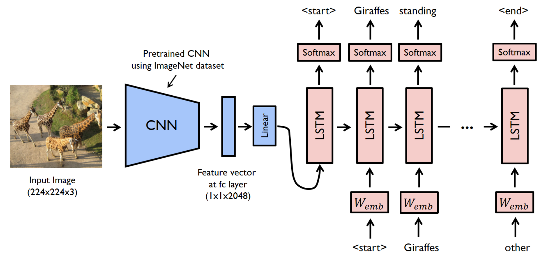
Fig. 11.3 CNN-RNN (Source: [Murphy, 2022], Chapter 15)#
11.1.2. Sequence Classification#
If we now presume to have a fixed-length output vector but with a variable-length sequence as input, then we mathematically seek to learn
this is called a seq2vec model. Here we presume the output \(y\) to be a class label.
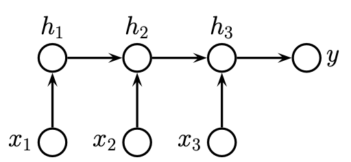
Fig. 11.4 Sequence to vector task (Source: [Murphy, 2022], Chapter 15)#
In its simplest form, we can just use the final state of the RNN as the input to the classifier
While this simple form can already produce good results, the RNN principle can be extended further by allowing information to flow in both directions, i.e., we allow the hidden states to depend on past and future contexts. For this, we have to use two basic RNN building blocks to then assemble them into a bidirectional RNN.
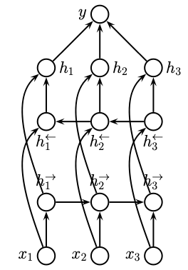
Fig. 11.5 Bi-directional RNN for seq2vec tasks (Source: [Murphy, 2022], Chapter 15)#
This bi-directional model is then defined as
where the hidden state then transforms into a vector of forward-, and reverse-time hidden state
One has to then average the pool over these states to arrive at the predictive model
11.1.3. Sequence Translation#
In sequence translation, we have a variable length sequence as an input and a variable length sequence as an output. This can mathematically be expressed as
For ease of notation, this has to be broken down into two subcases:
\(T'=T\), i.e., we have the same length of input- and output-sequences
\(T' \neq T\), i.e,. we have different lengths between the input- and the output-sequence
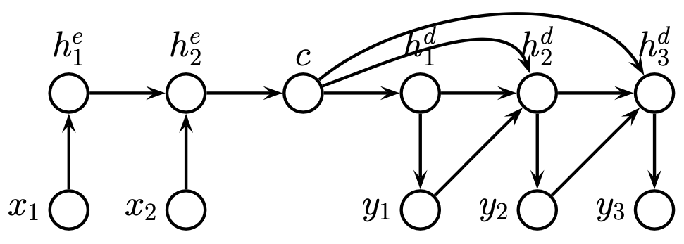
Fig. 11.6 Encoder-Decoder RNN for sequence-to-sequence task (Source: [Murphy, 2022], Chapter 15)#
11.1.3.1. Aligned Sequences#
We begin by examining the case for \(T'=T\), i.e. with the same length of input-, and output-sequences. In this case, we have to predict one label per location and can hence modify our existing RNN for this task
Once again, results can be improved by allowing for bi-directional information flow with a bidirectional RNN which can be constructed as shown before, or by stacking multiple layers on top of each other and creating a deep RNN.
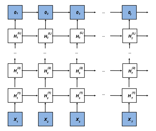
Fig. 11.7 Deep RNN (Source: [Murphy, 2022], Chapter 15)#
In the case of stacking layers on top of each other to create deeper networks, we have hidden layers lying on top of hidden layers. The individual layers are then computed with
and the output is computed from the final layer
11.1.3.2. Unaligned Sequences#
In the unaligned case, we have to learn a mapping from the input sequence to the output sequence, where we first have to encode the input sequence into a context vector
using the last state of an RNN or pooping over all states. We then generate the output sequence using a decoder RNN, which leads to the so-called encoder-decoder architecture. A plethora of tokenizers exist to construct the context vectors, and a plethora of decoding approaches, such as greedy decoding, are shown below.
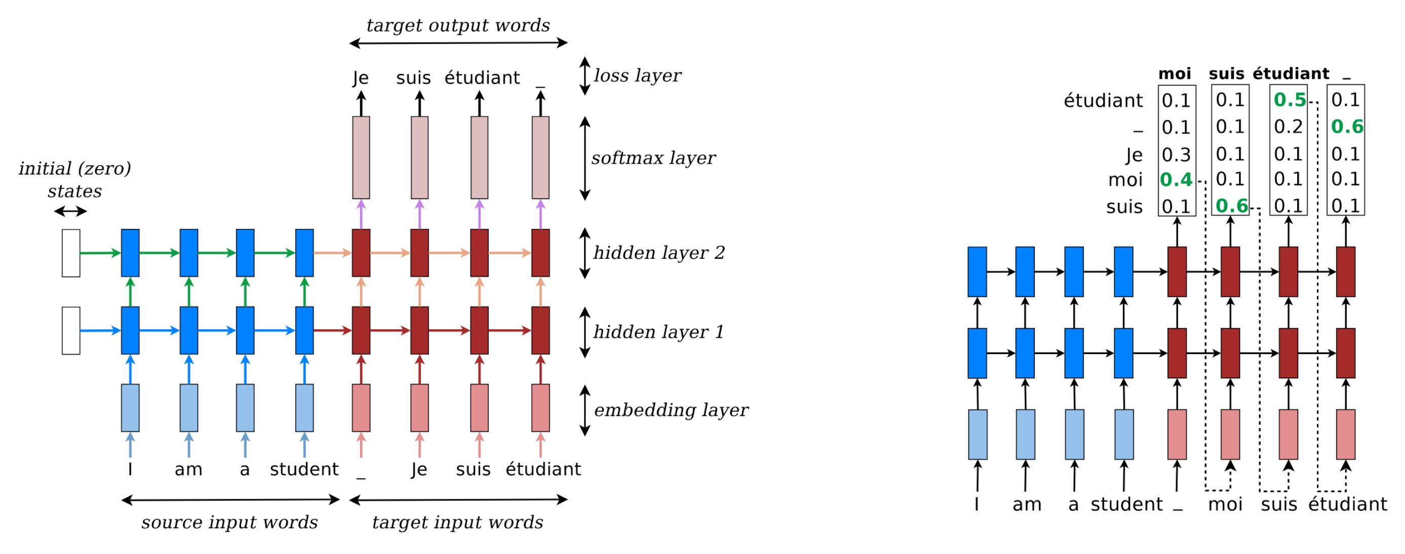
Fig. 11.8 Sequence to sequence translation of English to French using greedy decoding (Source: [Murphy, 2022], Chapter 15)#
This encoder-decoder architecture dominates general machine learning and scientific machine learning. Examining the use cases you have seen up to now:
U-Net
Convolutional LSTM, i.e., encoding with CNNs, propagating in time with the LSTM, and then decoding with CNNs again
Sequence Translation as just now
And an unending list of applications which you have seen in practice but have not seen in the course yet
Transformer models
GPT
BERT
ChatGPT
Diffusion models for image generation
…
But if RNNs can already do so much, why are Transformers then dominating machine learning research these days and not RNNs?
Training RNNs is far from trivial, with a well-known problem being exploding gradients, and vanishing gradients. In both cases, the activations of the RNN explode or decay as we go forward in time as we multiply with the weight matrix \(W_{hh}\) at each time step. The same can happen as we go backward in time, as we repeatedly multiply the Jacobians, and unless the spectrum of the Hessian is 1, this will result in exploding or vanishing gradients. A way to tackle this is via control of the spectral radius, where the optimization problem gets converted into a convex optimization problem, which is then called an echo state network. Which is in literature often used under the umbrella term of reservoir computing.
11.2. Long Short-term Memory (LSTM)#
A way to avoid the problem of exploding and vanishing gradients beyond Gated Recurrent Units (GRU), which we omit in this course, is the long short-term memory (LSTM) model of Schmidhuber and Hochreiter, back in the day at TUM. In the LSTM the hidden state \(h\) is augmented with a memory cell \(c\). This cell is then controlled with 3 gates
Output gate \(O_{t}\)
Input gate \(I_{t}\)
Forget gate \(F_{t}\)
where the forget gate determines when the memory cell is to be reset. The individual cells are then computed as
from which the cell state can then be computed as
with the actual update then given by either the candidate cell, if the input gate permits it, or the old cell, if the not-forget gate is on
The hidden state is then computed as a transformed version of the memory cell if the output gate is on
Visually this then looks like the following:
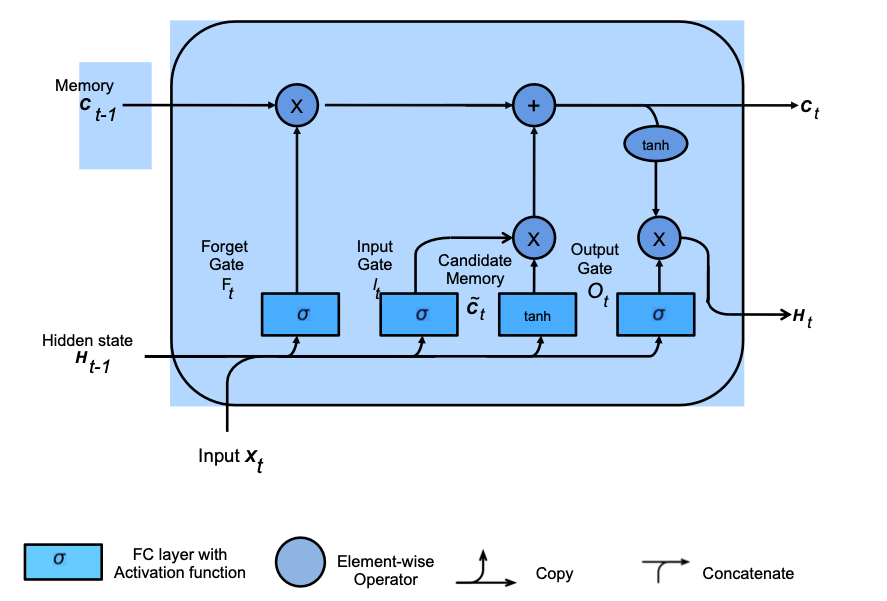
Fig. 11.9 LSTM block (Source: [Murphy, 2022], Chapter 15)#
This split results in the following properties:
\(H_{t}\) acts as a short-term memory
\(C_{t}\) acts as a long-term memory
In practice, this then takes the following form in code:
def lstm(inputs, state, params):
    [W_xi, W_hi, b_i, W_xf, W_hf, b_f, W_xo, W_ho, b_o, W_xc, W_hc, b_c, W_hq, b_q] = params
    (H, C) = state
    outputs = []
    for X in inputs:
        I = torch.sigmoid((X @ W_xi) + (H @ W_hi) + b_i)
        F = torch.sigmoid((X @ W_xf) + (H @ W_hf) + b_f)
        O = torch.sigmoid((X @ W_xo) + (H @ W_ho) + b_o)
        C_tilda = torch.tanh((X @ W_xc) + (H @ W_hc) + b_c)
        C = F * C + I * C_tilda
        H = O * torch.tanh(C)
        Y = (H @ W_hq) + b_q
        outputs.append(Y)
    return torch.cat(outputs, dim=0), (H, C)
There are variations of this initial architecture, but the core LSTM architecture and performance have prevailed over time. A different approach to sequence generation is using causal convolutions with 1-dimensional CNNs. While this approach has shown promise in quite a few practical applications, we view it as not relevant to the exam.
11.3. Advanced Topics: 1-Dimensional CNNs#
While RNNs have very strong temporal prediction abilities with their memory, as well as stateful computation, 1-D CNNs can constitute a viable alternative as they don’t have to carry along the long-term hidden state, as well as being easier to train as they do not suffer from exploding or vanishing gradients.
11.3.1. Sequence Classification#
Recalling, for sequence classification, we consider the seq2vec case, in which we have a mapping of the form
A 1-D convolution applied to an input sequence of length \(T\), and \(D\) features per input then takes the form
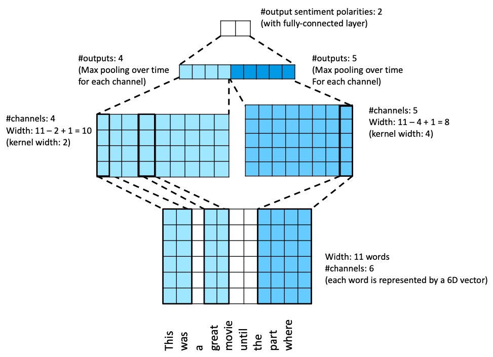
Fig. 11.10 TextCNN architecture (Source: [Murphy, 2022], Chapter 15)#
With \(D>1\) input channels of each input sequence, each channel is then convolved separately, and the results are then added up with each channel having its own separate 1-D kernel s.t. (recalling from the CNN lecture)
with \(k\) being the size of the receptive field, and \(w_{d}\) the filter for the input channel \(d\). Which produces a 1-D input vector \(z \in \mathbb{R}^{T}\) (ignoring boundaries), i.e. for each output channel \(c\) we then get
To then reduce this to a fixed size vector \(z \in \mathbb{R}^{C}\), we have to use max-pooling over time s.t.
which is then passed into a softmax layer. What this construction permits is that by choosing kernels of different widths, we can essentially use a library of different filters to capture patterns of different frequencies (length scales). In code, this then looks the following:
class TextCNN(nn.Module):
    def __init__(self, vocab_size, embed_size, kernel_sizes, num_channels, **kwargs):
        super(TextCNN, self).__init__(**kwargs)
        self.embedding = nn.Embedding(vocab_size, embed_size)
        self.constant_embedding = nn.Embedding(vocab_size, embed_size) # not being trained
        self.dropout = nn.Dropout(0.5)
        self.decoder = nn.Linear(sum(num_channels), 2)
        self.pool = nn.AdaptiveAvgPool1d(1)  # no weight and can hence share the instance
        self.relu = nn.ReLU()
        # Creating the one-dimensional convolutional layers with different kernel widths
        self.convs = nn.ModuleList()
        for c, k in zip(num_channels, kernel_sizes):
            self.convs.append(nn.Conv1d(2 * embed_size, c, k))

    def forward(self, inputs):
        # Concatenation of the two embedding layers
        embeddings = torch.cat((self.embedding(inputs), self.constant_embedding(inputs)), dim=2)
        # Channel dimension of the 1-D conv layer is transformed
        embeddings = embeddings.permute(0, 2, 1)
        # Flattening to remove overhanging dimension, and concatenate on the channel dimension
        # For each one-dimensional convolutional layer, after max-over-time
        encoding = torch.cat(
            [torch.squeeze(self.relu(self.pool(conv(embeddings))), dim=-1) for conv in self.convs], dim=1
        )
        outputs = self.decoder(self.dropout(encoding))
        return outputs
11.3.2. Sequence Generation#
To use CNNs generatively, we need to introduce causality into the model, this results in the model definition of
where we have the convolutional filter \(w\) and a nonlinearity \(\varphi\). This results in a masking out of future inputs, such that \(y_{t}\) can only depend on past information and no future information. This is called a causal convolution. One poster-child example of this approach is the WaveNet architecture, which takes in text as input sequences to generate raw audio such as speech. The WaveNet architecture utilizes dilated convolutions in which the dilation increases with powers of 2 with each successive layer.
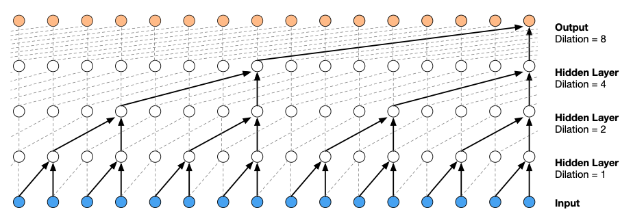
Fig. 11.11 WaveNet architecture (Source: [Murphy, 2022], Chapter 15)#
This then takes the following form in code.
11.4. Flagship Applications#
With so many flagship models of AI these days relying on sequence models, we have compiled a list of very few of them below for you to play around with. While attention was beyond the scope of this lecture, you can have a look at Lilian Weng’s blog post on attention below to dive into it.
Large Language Models (LLMs)
ChatGPT: Optimizing Language Models for Dialogue
GPT-3 - where ChatGPT started
BERT - Google’s old open-source LLM
Llama 2 - Meta’s open source LLMs
Mistral/Mixtral - Mistral AI’s open source LLMs
Others
OpenAI’s Dall-E 2 - image generation
Stable Diffusion - open source image generation
Whisper - open source audio-to-text model
11.5. Further Reading#
[Murphy, 2022], Chapter 15 - main reference for this lecture