Support Vector Machines

6. Support Vector Machines#

Learning outcome

What are Lagrange multipliers in the context of constrained optimization?
Explain how the decision boundary of the maximum margin classifier depends on each data point. Illustrate your explanation with a drawing.
How does the kernel method allow us to separate otherwise not linearly separable data points?
When is a kernel valid?

Support Vector Machines are one of the most popular classic supervised learning algorithms. This lecture will first discuss the mathematical formalism of solving constrained optimization problems using Lagrange multipliers. We will then look at linear binary classification using the maximum margin and soft margin classifiers. Ultimately, we will present the kernel trick and how it extends the previous two approaches to non-linear boundaries within the more general Support Vector Machine.

6.1. The Constrained Optimization Problem#

We define a constrained optimization problem as

(6.1)#

min_{ω} f (ω) s.t. h_{i} (ω) = 0, i = 1, \dots, l

Here, $min_{ω}$ seeks to find the minimum subject to the constraint(s) $h_{i} (ω)$ . One possible way to solve this is to use Lagrange multipliers, for which we define the Lagrangian $L$ , which takes the constraints into account.

(6.2)#

L (ω, β) = f (ω) + \sum_{i = 1}^{l} β_{i} h_{i} (ω) .

The $β_{i}$ are the Lagrangian multipliers, which need to be identified to find the constraint-satisfying $ω$ . The necessary conditions to solve this problem are to solve

(6.3)#

\frac{\partial L}{\partial ω_{i}} = 0; \frac{\partial L}{\partial β_{i}} = 0,

for $ω$ and $β$ . In classification problems, we do not only have equality constraints as above but can also encounter inequality constraints. We formulate the general primal optimization problem as:

(6.4)#

\begin{array}{r} min_{ω} f (ω) s.t. {\begin{cases} g_{i} (ω) \leq 0, i = 1, \dots, k, \\ h_{i} (ω) = 0, i = 1, \dots, l . \end{cases} \end{array}

To solve it, we define the generalized Lagrangian.

(6.5)#

L (ω, α, β) = f (ω) + \sum_{i = 1}^{k} α_{i} g_{i} (ω) + \sum_{i = 1}^{l} β_{i} h_{i} (ω),

with the additional Lagrange multipliers $α_{i}$ . Let us define the primal quantity

(6.6)#

θ_{P} (ω) = max_{α_{i} \geq 0, β_{j}} L (ω, α, β) .

Now, we can verify that this optimization problem satisfies

(6.7)#

\begin{array}{r} θ_{P} (ω) = {\begin{cases} f (ω) if ω satisfies the primal constraints, \\ \infty otherwise . \end{cases} \end{array}

Where does this case-by-case breakdown come from?

In the first case, the constraints are inactive and contribute nil to the sum.
In the second case, the sums increase linearly with $α_{i}$ , $β_{i}$ beyond all bounds.

(6.8)#

⟹ p^{⋆} = min_{ω} θ_{P} (ω) = min_{ω} max_{α_{i} \geq 0, β_{j}} L (ω, α, β) .

That is, we recover the original primal problem with $p^{⋆}$ being the optimal value of the primal problem. With this, we can now formulate the dual optimization problem:

(6.9)#

d^{⋆} = max_{α_{i} \geq 0, β_{j}} θ_{D} (α, β) = max_{α_{i} \geq 0, β_{j}} min_{ω} L (ω, α, β),

with $θ_{D} (α, β) = min_{ω} L (ω, α, β)$ and $d^{⋆}$ the optimal value of the dual problem. Please note that the primal and dual problems are equivalent to exchanging the order of minimization and maximization. To show how these problems are related, we first derive a relation between min-max and max-min using $μ (y) = inf_{x} κ (x, y)$ :

(6.10)#

\begin{array}{r} \begin{aligned} ⟹ μ (y) \leq κ (x, y) \\ ⟹ sup_{y} μ (y) \leq sup_{y} κ (x, y) \\ ⟹ sup_{y} μ (y) \leq inf_{x} sup_{y} κ (x, y) \\ ⟹ sup_{y} inf_{x} κ (x, y) \leq inf_{x} sup_{y} κ (x, y) \end{aligned} \end{array}

From the last line, we can immediately imply the relation between the primal and the dual problems.

(6.11)#

d^{⋆} = max_{α_{i} \geq 0, β_{j}} min_{ω} L (ω, α, β) \leq min_{ω} max_{α_{i} \geq 0, β_{j}} L (ω, α, β) = p^{⋆},

where the inequality can, under certain conditions, turn into equality. The conditions for this to become equality are the following (going back to the Lagrangian form from above):

$f$ and $g_{i}$ are convex, i.e. their Hessians are positive semi-definite.
The $h_{i}$ are affine, i.e., they can be expressed as linear functions of their arguments.

Under the above conditions, the following holds:

The optimal solution $ω^{⋆}$ to the primal optimization problem exists.
The optimal solution $α^{⋆}$ , $β^{⋆}$ to the dual optimization problem exists.
$p^{⋆} = d^{⋆}$ .
$ω^{⋆}$ , $α^{⋆}$ , and $β^{⋆}$ satisfy the Karush-Kuhn-Tucker (KKT) conditions.

The KKT conditions are expressed as the following conditions:

(6.12)#

\begin{array}{r} \begin{aligned} {\frac{\partial L (ω, α, β)}{\partial ω_{i}} |}_{ω^{⋆}, α^{⋆}, β^{⋆}} & = 0, i = 1, \dots, n & (KKT1) \\ {\frac{\partial L (ω, α, β)}{\partial β_{i}} |}_{ω^{⋆}, α^{⋆}, β^{⋆}} & = 0, i = 1, \dots, l & (KKT2) \\ α_{i}^{⋆} g_{i} (ω^{⋆}) & = 0, i = 1, \dots, k & (KKT3) \\ g_{i} (ω^{⋆}) & \leq 0, i = 1, \dots, k & (KKT4) \\ α_{i}^{⋆} & \geq 0, i = 1, \dots, k & (KKT5) \end{aligned} \end{array}

Moreover, if a set ${ω^{⋆}$ , $α^{⋆}, β^{⋆}}$ satisfies the KKT conditions, then it is a solution to the primal/dual problem. The KKT conditions are sufficient and necessary here. The dual complementarity condition (KKT3) indicates whether the $g_{i} (ω) \leq 0$ constraint is active:

(6.13)#

α_{i}^{⋆} > 0 ⟹ g_{i} (ω^{⋆}) = 0,

i.e., if $α_{i}^{⋆} > 0$ , then $ω^{⋆}$ is “on the constraint boundary”.

6.2. Maximum Margin Classifier (MMC)#

Alternative names for Maximum Margin Classifier (MMC) are Hard Margin Classifier and Large Margin Classifier. This classifier assumes that the classes are linearly separable.

Now, we can (re-)introduce the linear discriminator. As we have seen, logistic regression $p (y = 1 | x; ϑ)$ is modeled by $h (x) = g (ϑ^{⊤} x) = sigmoid (ϑ^{⊤} x)$ :

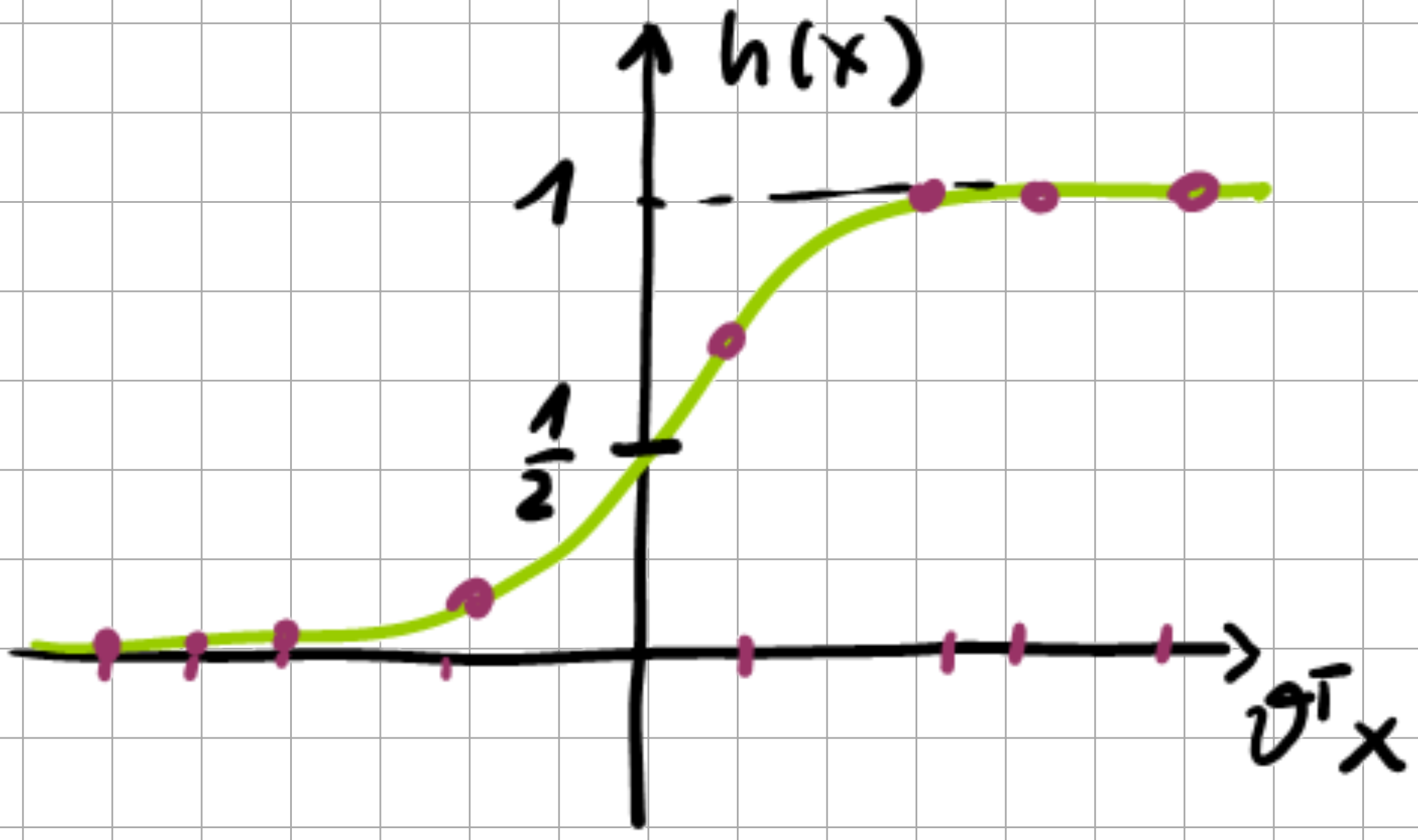
../_images/sigmoid_svm.png — Fig. 6.1 Sigmoid function.#

If $g (ϑ^{⊤} x)$ is close to one, then we have large confidence that $x$ belongs to class $C_{1}$ with $y = 1$ , whereas if it is close to $\frac{1}{2}$ , we have much less confidence:

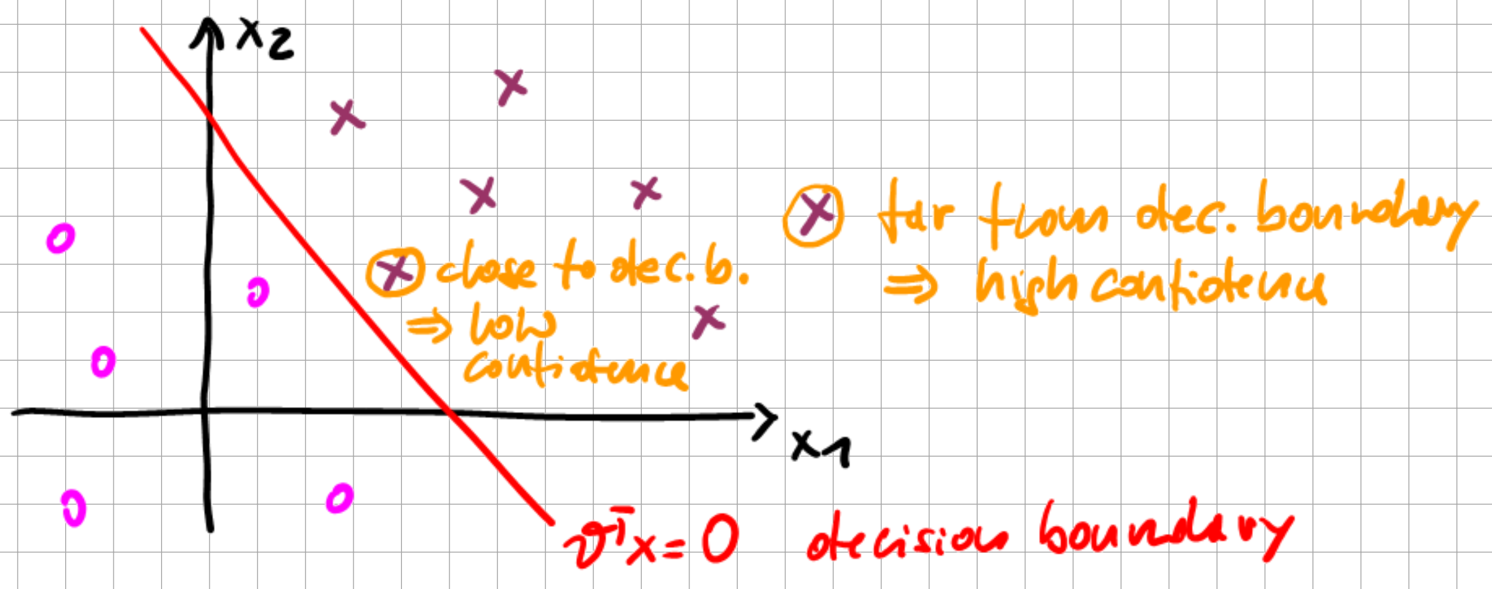
../_images/log_reg_confidence.png — Fig. 6.2 Confidence of logistic regression classifier.#

The intuition here is that we seek to find the model parameters $ϑ$ such that $g (ϑ^{⊤} x)$ maximizes the distance from the decision boundary $g (ϑ^{⊤} x) = \frac{1}{2}$ for all data points.

For consistency with the standard SVM notation, we slightly reformulate this problem setting:

(6.14)#

\begin{array}{r} \begin{aligned} y & \in {- 1, 1} as binary class labels \\ h (x) & = g (ω^{⊤} x + b) as classifier with \\ g (z) & = {\begin{cases} 1, z \geq 0 \\ - 1, z < 0, \end{cases} \end{aligned} \end{array}

where $ω^{⊤} x + b$ defines a hyperplane for our linear classifier. With $b$ , we now make the bias explicit, as it was previously implicit in our expressions.

6.2.1. Functional Margin#

The functional margin of $(ω, b)$ w.r.t. a single training sample is defined as

(6.15)#

{\hat{γ}}^{(i)} = y^{(i)} (ω^{⊤} x^{(i)} + b) .

For a confident prediction, we would then like to have a maximum gap between the classes for a good classifier.

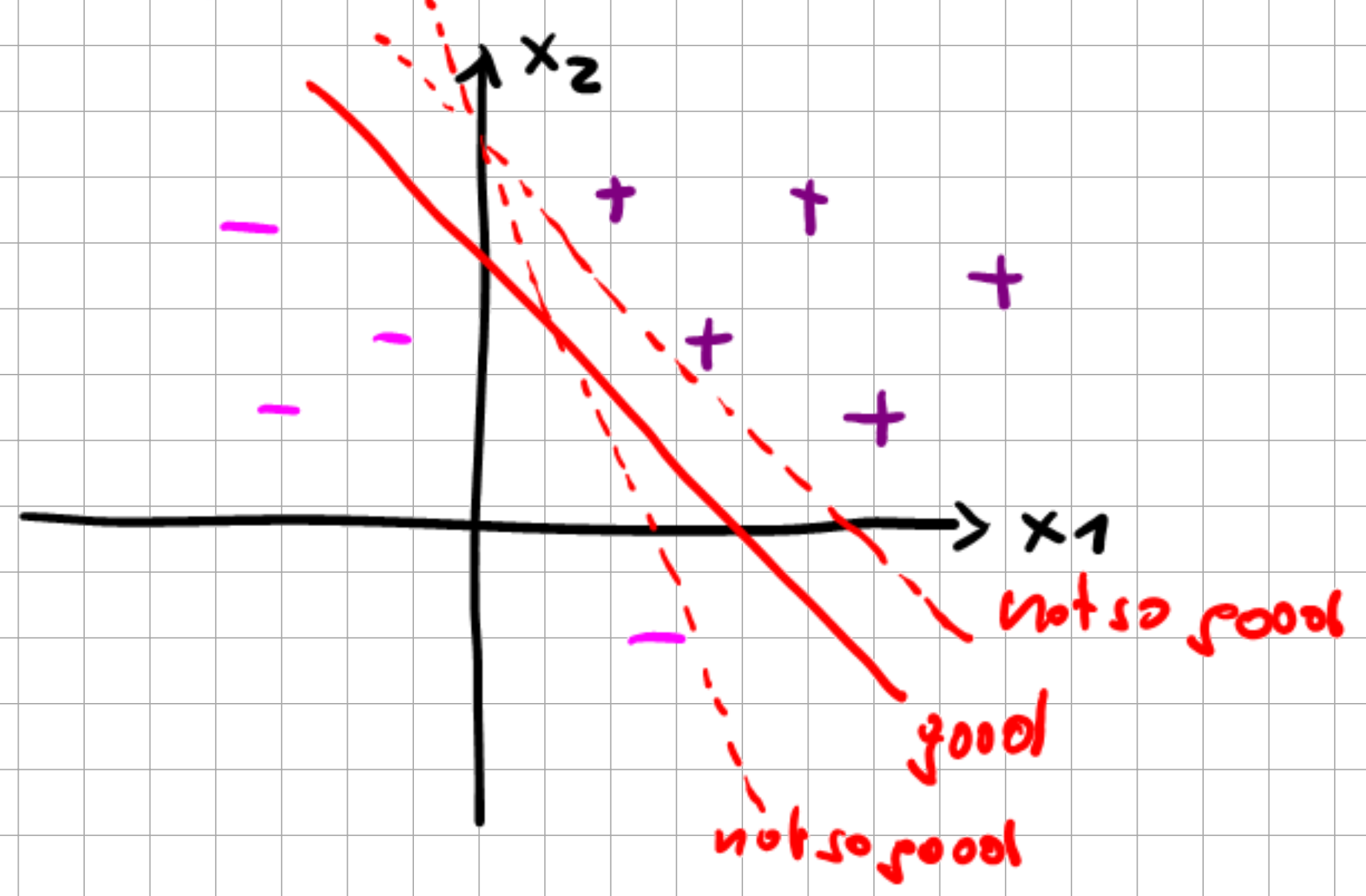
../_images/good_vs_bad_classifier_svm.png — Fig. 6.3 Good vs bad linear decision boundary.#

For correctly classified samples, we always have

(6.16)#

y^{(i)} (ω^{⊤} x^{(i)} + b) > 0

as $g (ω^{⊤} x + b) = y = \pm 1$ . Note that the induced functional margin is invariant to scaling:

(6.17)#

g (ω^{⊤} x + b) = g (2 ω^{⊤} x + 2 b) = \dots

However, if we want to maximize this margin, we could do that without changing the actual decision boundary. Also, note that the classifier does not reflect that the margin is not invariant.

For the entire set of training samples, we define the functional margin as

(6.18)#

\hat{γ} = min_{i} {\hat{γ}}^{(i)} .

6.2.2. Geometric Margin#

Now we can define the geometric margin with respect to a single sample $γ^{(i)}$ as follows.

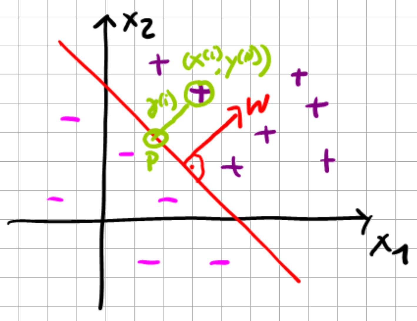
../_images/geometric_margin.png — Fig. 6.4 The geometric margin.#

The distance $γ^{(i)}$ of point $x^{(i)}$ from the decision boundary, i.e., from the closest point P on that boundary, is given by

(6.19)#

ω^{⊤} (x^{(i)} - γ^{(i)} \frac{ω}{| | ω | |}) + b = 0,

where $x^{(i)} - γ^{(i)} \frac{ω}{| | ω | |}$ gives the location of the point P, and $\frac{ω}{| | ω | |}$ is the unit normal. As P is a member of the decision boundary, no matter where it is placed on the boundary, the equality always has to be zero by definition.

(6.20)#

⟹ γ^{(i)} = {(\frac{ω}{| | ω | |})}^{⊤} x^{(i)} + \frac{b}{| | ω | |} .

As this was for an example on the $+$ side, we can generalize said expression to obtain

(6.21)#

γ^{(i)} = y^{(i)} ({(\frac{ω}{| | ω | |})}^{⊤} x^{(i)} + \frac{b}{| | ω | |}) .

Please note that the geometric margin indeed is scale invariant. Also, note that for $| | ω | | = 1$ the functional and geometric margin are the same. For the entire set of samples, we can then define the geometric margin as:

(6.22)#

γ = min_{i} γ^{(i)} .

6.2.3. Maximum Margin Classifier#

With these mathematical tools, we are now ready to derive the Support Vector Machine (SVM) for linearly separable sets (a.k.a. Maximum Margin Classifier) by maximizing the previously derived geometric margin:

(6.23)#

\begin{array}{r} max_{γ, ω, b} γ s.t. {\begin{cases} y^{(i)} (ω^{⊤} x^{(i)} + b) \geq γ, i = 1, \dots, m \\ | | ω | | = 1 ⟹ \hat{γ} = γ . \end{cases} \end{array}

However, in this formulation, the second constraint $| | ω | | = 1$ is non-convex, which is inefficient to solve numerically. Thus, we formulate a slightly different optimization problem that again seeks to maximize the geometric margin:

(6.24)#

max_{\hat{γ}, ω, b} \frac{\hat{γ}}{| | ω | |} s.t. y^{(i)} (ω^{⊤} x^{(i)} + b) \geq \hat{γ}, i = 1, \dots, m,

where we applied the definition of $γ = \frac{\hat{γ}}{| | ω | |}$ . Although we eliminated the previous non-convex constraint, we suffered a setback in the process as we now have a non-convex objective function. In a third attempt to formulate an optimization problem, using that the geometric margin $γ$ is scale-invariant, we can now simply scale $| | ω | |$ such that $\hat{γ} = γ | | ω | | = 1$ . Given $\hat{γ} = 1$ it is clear that

(6.25)#

max_{\hat{γ}, ω, b} \frac{\hat{γ}}{| | ω | |} = max_{ω, b} \frac{1}{| | ω | |} = min_{ω, b} | | ω | |^{2},

s.t. the constraints are satisfied. This is now a convex objective with linear constraints.

The Support Vector Machine is generated by the primal optimization problem.

(6.26)#

min_{ω, b} \frac{1}{2} | | ω | |^{2} s.t. y^{(i)} (ω^{⊤} x^{(i)} + b) \geq 1, i = 1, \dots, m,

or alternatively

(6.27)#

min_{ω, b} \frac{1}{2} | | ω | |^{2} s.t. g_{i} (ω) = 1 - y^{(i)} (ω^{⊤} x^{(i)} + b) \leq 0, i = 1, \dots, m .

Upon checking with the KKT dual complementarity condition, we see that $α_{i} > 0$ only for samples with $γ_{i} = 1$ , i.e.

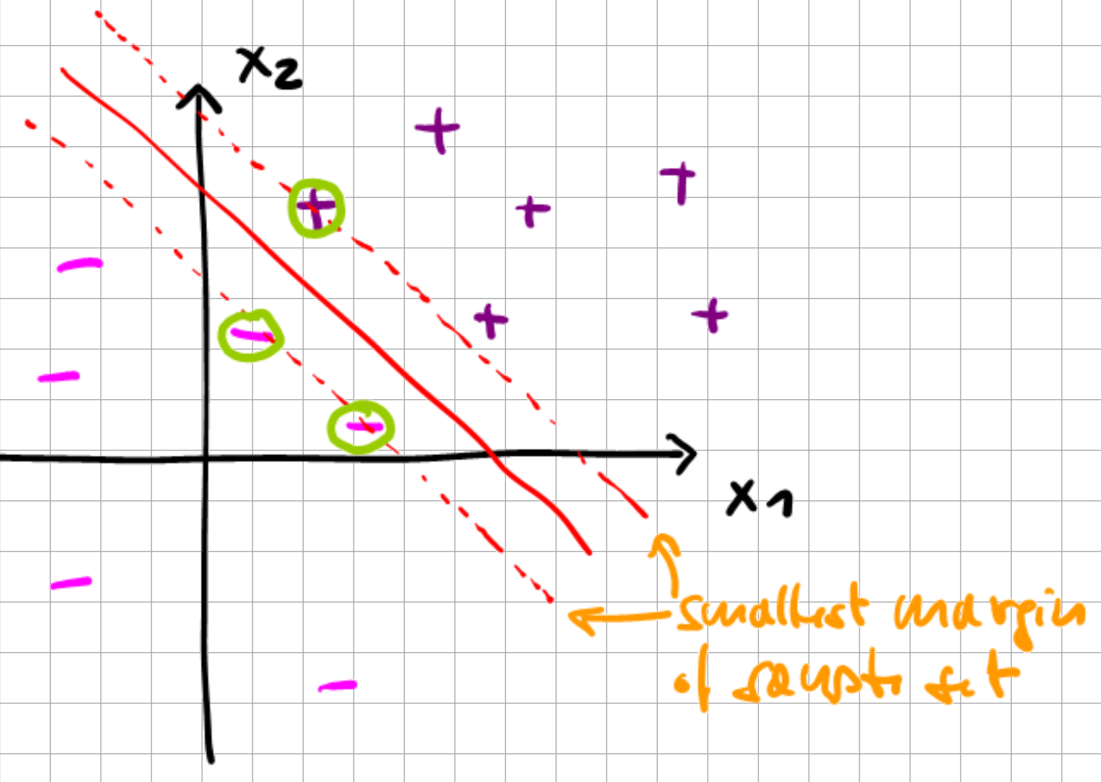
../_images/maximum_margin_classifier.png — Fig. 6.5 Maximum Margin Classifier.#

The three samples “-”, “-”, and “+” in the sketch are the only ones for which the KKT constraint is active.

These are called the support vectors.

From the sketch, we can already ascertain that the number of support vectors may be significantly smaller than the number of samples, i.e., the number of active constraints that we have to take into account. Next, we construct the Lagrangian of the optimization problem:

(6.28)#

L (ω, b, α) = \frac{1}{2} | | ω | |^{2} - \sum_{i = 1}^{m} α_{i} [y^{(i)} (ω^{⊤} x^{(i)} + b) - 1]

Note that in this case, our Lagrangian only has inequality constraints!

We can then formulate the dual problem $θ_{D} (α) = min_{ω, b} L (ω, b, α)$ and solve for $ω$ and $b$ by setting the derivatives to zero.

(6.29)#

\begin{array}{r} \begin{aligned} \nabla_{ω} L (ω, b, α) & = ω - \sum_{i = 1}^{m} α_{i} y^{(i)} x^{(i)} = 0 \\ ⟹ ω & = \sum_{i = 1}^{m} α_{i} y^{(i)} x^{(i)} \\ ⟹ \frac{\partial L}{\partial b} & = \sum_{i = 1}^{m} α_{i} y^{(i)} = 0. \end{aligned} \end{array}

The $ω$ we can then resubstitute into the original Lagrangian (Eq. (6.28)) to get the term

(6.30)#

\sum_{i = 1}^{m} α_{i} y^{(i)} ω^{⊤} x^{(i)} = ω^{⊤} \sum_{i = 1}^{m} α_{i} y^{(i)} x^{(i)} = ω^{⊤} ω = | | ω | |^{2} .

If we plug that into the Lagrangian (Eq. (6.28)), we get the dual

(6.31)#

\begin{array}{r} \begin{aligned} θ_{D} (α) & = - \frac{1}{2} | | ω | |^{2} + \sum_{i = 1}^{m} α_{i} - b \sum_{i = 1}^{m} α_{i} y^{(i)} \\ = - \frac{1}{2} | | ω | |^{2} + \sum_{i = 1}^{m} α_{i} (by the derivative w.r.t. b) \\ = \sum_{i = 1}^{m} α_{i} - \frac{1}{2} \sum_{i, j = 1}^{m} y^{(i)} y^{(j)} α_{i} α_{j} x^{(i)^{⊤}} x^{(j)}, \end{aligned} \end{array}

which we can then optimize as an optimization problem

(6.32)#

\begin{array}{r} max_{α} θ_{D} (α) s.t. {\begin{cases} α_{i} \geq 0, i = 1, \dots, m \\ \sum_{i = 1}^{m} α_{i} y^{(i)} = 0. \end{cases} \end{array}

The first constraint in this optimization problem singles out the support vectors, whereas the second constraint derives itself from our derivation of the dual of the Lagrangian (see above). The KKT conditions are then also satisfied.

The first KKT condition is satisfied as of our first step in the conversion to the Lagrangian dual.
The second KKT condition is not relevant.
The third KKT condition is satisfied with $α_{i} > 0 \Leftrightarrow y^{(i)} (ω^{⊤} x^{(i)} + b) = 0$ , i.e. the support vectors, and $α_{i} = 0 \Leftrightarrow y^{(i)} (ω^{⊤} x^{(i)} + b) < 1$ for the others.
The fourth KKT condition $y^{(i)} (ω^{⊤} x^{(i)} + b) \leq 1$ is satisfied by our construction of the Lagrangian.
The fifth KKT condition $α_{i} \geq 0$ is satisfied as of our dual optimization problem formulation.

⟹ d^{⋆} = p^{⋆}, i.e. the dual problem solves the primal problem.

The two then play together in the following fashion:

The dual problem gives $α^{⋆}$
The primal problem gives $ω^{⋆}$ , $b^{⋆}$ , with $b^{⋆}$ given by

(6.33)#

b^{⋆} = - \frac{max_{i \in C_{2}} ω^{⋆^{⊤}} x^{(i)} + min_{j \in C_{1}} ω^{⋆^{⊤}} x^{(j)}}{2}

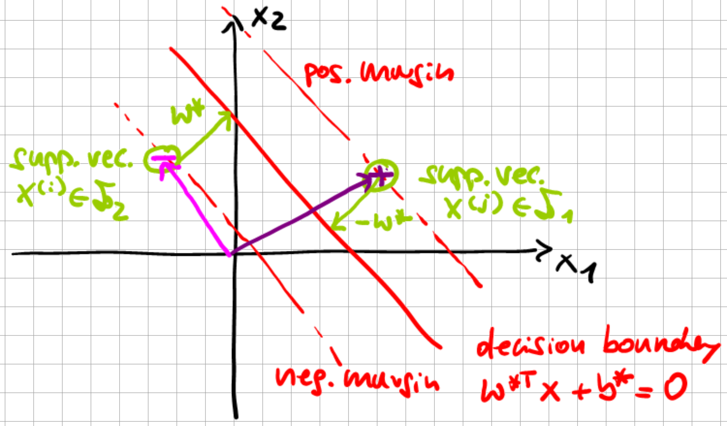
../_images/maximum_margin_classifier_solution.png — Fig. 6.6 Maximum Margin Classifier solution.#

To derive $b^{⋆}$ , we start from $x^{(i)}$ on the negative margin. One then gets to the decision boundary by $x^{(i)} + ω^{⋆}$ , and from $x^{(j)}$ on the positive margin by $x^{(j)} - ω^{⋆}$ , i.e.

(6.34)#

\begin{array}{r} \begin{aligned} ⟹ max_{i \in C_{2}} ω^{⋆^{⊤}} x^{(i)} + ω^{⋆^{⊤}} ω^{⋆} + b^{⋆} & = 0 \\ min_{j \in C_{1}} ω^{⋆^{⊤}} x^{(j)} - ω^{⋆^{⊤}} ω^{⋆} + b^{⋆} & = 0 \end{aligned} \end{array}

As $ω^{⋆^{⊤}} ω^{⋆} = 1$ , we can then solve for $b^{⋆}$ and obtain the result in Eq. (6.33). Now we can check how the SVM predicts $y$ given $x$ :

(6.35)#

\begin{array}{r} \begin{aligned} ω^{⋆^{⊤}} x + b^{⋆} & = {(\sum_{i = 1}^{m} α_{i}^{⋆} y^{(i)} x^{(i)})}^{⊤} x + b^{⋆} \\ = \sum_{i = 1}^{m} α_{i}^{⋆} y^{(i)} ⟨ x^{(i)}, x ⟩ + b^{⋆}, \end{aligned} \end{array}

where $α_{i}$ is only non-zero for support vectors and calls the inner product $⟨ x^{(i)}, x ⟩$ , which is hence a highly efficient computation. We have derived the support vector machine for the linear classification of sets. The formulation of the optimal set-boundary/decision boundary was formulated as the search for a margin optimization, then transformed into a convex, constrained optimization problem before restricting the contributions of the computation to contributions coming from the support vectors, i.e., vectors on the actual decision boundary estimate hence leading to a strong reduction of the problem dimensionality.

6.3. Advanced Topics: Soft Margin Classifier (SMC)#

What if the data is not linearly separable?

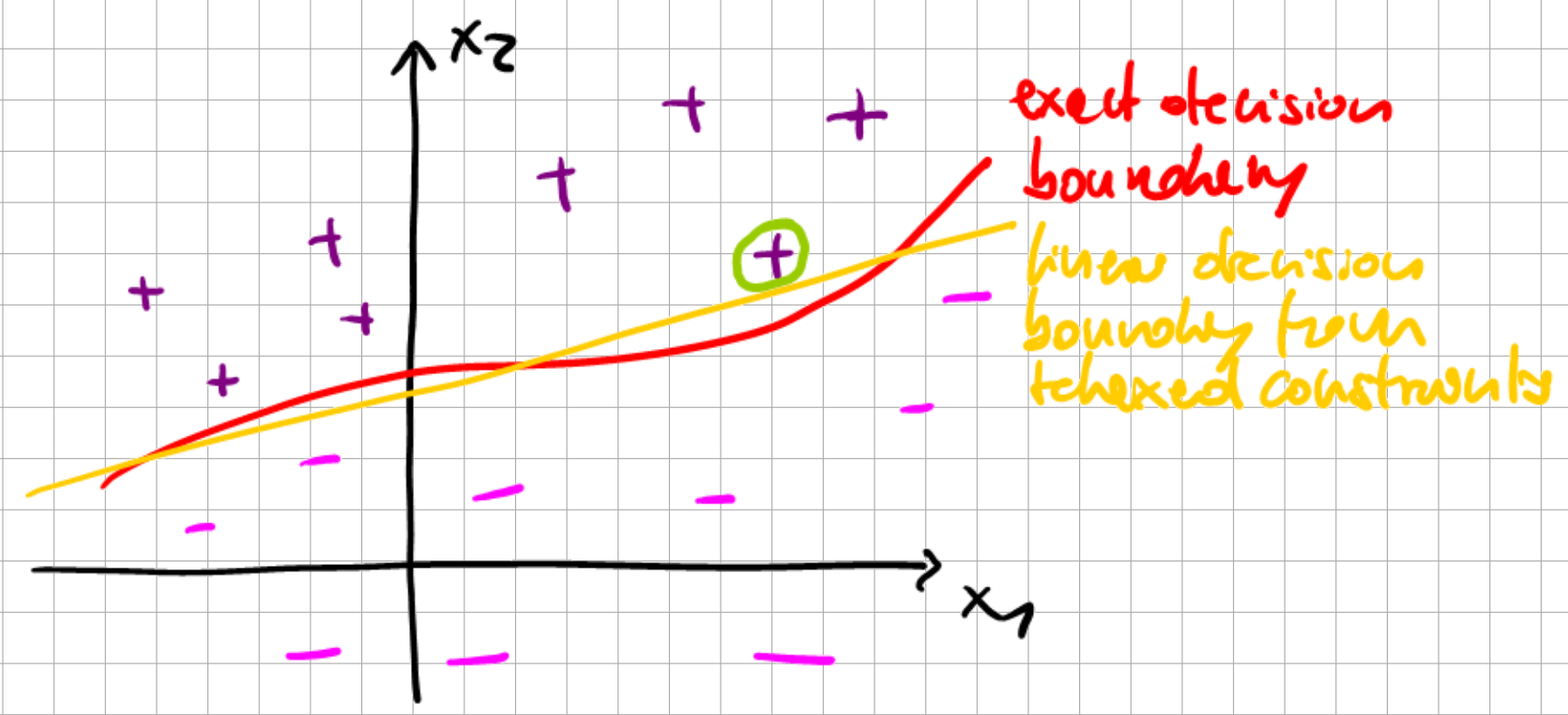
../_images/svm_nonlinearly_separable.png — Fig. 6.7 Non-linearly separable sets.#

Data may not be exactly linearly separable, or some data outliers may undesirably deform the exact decision boundary.

6.3.1. Outlier problem#

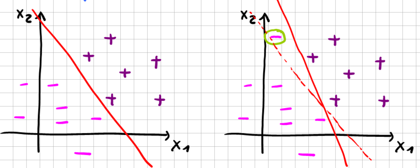
../_images/svm_sets_with_outlier.png — Fig. 6.8 Sensitivity of MMC to outliers.#

6.3.2. Original SVM optimization problem#

(6.36)#

min_{ω, b} \frac{1}{2} ‖ ω ‖^{2} s.t. y^{(i)} (ω^{⊤} x^{(i)} + b) \geq 1, i = 1, \dots, m

To make the algorithm work for non-linearly separable data, we introduce $l_{1}$ -regularization, i.e., a penalty term proportional to the magnitude of a certain quantity.

$\Rightarrow l_{1}$ -regularised primal optimization problem

min_{ω, b} \frac{1}{2} ‖ ω ‖^{2} + C \sum_{i = 1}^{m} ξ_{i}

(6.37)#

\begin{array}{r} s.t. {\begin{cases} y^{(i)} (ω^{⊤} x^{(i)} + b) \geq 1 - ξ_{i}, i = 1, \dots, m \\ ξ_{i} \geq 0, i = 1, \dots, m \end{cases} \end{array}

Here, $ξ_{i}$ is called a “slack” variable. We relax the previous requirement of a unit functional margin $\hat{γ} = 1$ by allowing some violation, which is penalized in the objective function.

margin ${\hat{γ}}^{(i)} = 1 - ξ_{i}, ξ_{i} > 0$
penalization $C ξ_{i}$
parameter $C$ controls the weight of the penalization

Then, the Lagrangian of the penalized optimization problem becomes

(6.38)#

L (ω, b, ξ, α, μ) = \frac{1}{2} ω^{T} ω + C \sum_{i = 1}^{m} ξ_{i} - \sum_{i = 1}^{m} α_{i} [y^{(i)} (ω^{⊤} x^{(i)} + b) - 1 + ξ_{i}] - \sum_{i = 1}^{m} μ_{i} ξ_{i} .

In the above equation, the second term ( $C \sum_{i = 1}^{m} ξ_{i}$ ) represents the soft penalization of strict margin violation, whereas the third and fourth terms are the inequality constraints with Lagrangian multipliers $α_{i}$ and $μ_{i}$ . The derivation of the dual problem follows from the analogous steps of the non-regularised SVM problem.

(6.39)#

\begin{array}{r} \begin{aligned} \frac{\partial L}{\partial ω} \overset{!}{=} 0 \Rightarrow w = \sum_{i = 1}^{m} α_{i} y^{(i)} x^{(i)} \\ \frac{\partial L}{\partial b} \overset{!}{=} 0 \Rightarrow \sum_{i = 1}^{m} α_{i} y^{(i)} = 0 \\ \frac{\partial L}{\partial ξ} \overset{!}{=} 0 \Rightarrow α_{i} = C - μ_{i}, i = 1, \dots, m (⋆) \end{aligned} \end{array}

The last equation arises from the additional condition due to slack variables. Upon inserting these conditions into $L (ω, b, ξ, α, μ)$ we obtain the dual-problem Lagrangian:

(6.40)#

\begin{array}{r} \begin{aligned} max_{α} θ_{D} (α) & = max_{α} (\sum_{i = 1}^{m} α_{i} - \frac{1}{2} \sum_{i, j = 1}^{m} y^{(i)} y^{(j)} α_{i} α_{j} ⟨ x^{(i)}, x^{(j)} ⟩) \\ s.t. & {\begin{matrix} 0 \leq α_{i} \leq C, i = 1, \dots, m \\ \sum_{i = 1}^{m} α_{i} y^{(i)} = 0 \end{matrix} \end{aligned} \end{array}

The “box constraints” ( $0 \leq α_{i} \leq C$ ) follow from the positivity requirement on Lagrange multipliers: $α_{i} \geq 0, μ_{i} \geq 0$ . Evaluating the KKT3-complementarity condition leads to

(6.41)#

\begin{array}{r} \begin{aligned} α_{i}^{*} [y^{(i)} (ω^{⊤} x^{(i)} + b) - 1 + ξ_{i}] = 0 \Leftrightarrow {\begin{cases} α_{i}^{*} > 0, & y^{(i)} (ω^{⊤} x^{(i)} + b) = 1 - ξ_{i} \\ α_{i}^{*} = 0, & y^{(i)} (ω^{⊤} x^{(i)} + b) \geq 1 - ξ_{i} \end{cases} \\ μ_{i}^{*} ξ_{i} = 0 \Leftrightarrow {\begin{cases} μ_{i}^{*} > 0, & ξ_{i} = 0 \\ μ_{i}^{*} = 0, & ξ_{i} > 0 \end{cases} \end{aligned} \end{array}

The resulting dual complementarity conditions for determining the support vectors become:

Support vectors on slack margin ( $α_{i} = 0$ , i.e. data point is ignored)

(6.42)#

α_{i}^{*} = 0 \Rightarrow y^{(i)} (ω^{⊤} x^{(i)} + b) \geq 1

Support vectors inside or outside margin ( $α^{*} = C$ , i.e. data point violates the MMC)

(6.43)#

\begin{array}{r} \begin{aligned} C = α_{i}^{*} & (⋆) \Rightarrow μ_{i}^{*} = 0, {\begin{array}{rr} 0 < ξ_{i} \leq 1 & (correctly classified) \\ ξ_{i} > 1 & (misclassified) \end{array} \\ \Rightarrow y^{(i)} (ω^{⊤} x^{(i)} + b) < 1 \end{aligned} \end{array}

Support vectors on margin ( $α_{i}^{*} > 0$ & $ξ_{i} > 0$ , i.e. data point on the margin)

(6.44)#

\begin{array}{r} \begin{aligned} 0 < α_{i}^{*} < C & (⋆) \Rightarrow μ_{i}^{*} > 0 \Rightarrow ξ_{i} = 0 \\ \Rightarrow y^{(i)} (ω^{⊤} x^{(i)} + b) = 1 \end{aligned} \end{array}

The optimal $b^{*}$ is obtained from averaging over all support vectors: condition to be satisfied by $b^{*}$ is given by SVs on the margin:

(6.45)#

0 < α_{i}^{*} < C \Rightarrow y^{(i)} (ω^{⊤} x^{(i)} + b) = 1

$\Rightarrow$ for $ω^{*}$ , we obtain the same result as for the linearly separable problem

(6.46)#

ω^{*} = \sum_{i = 1}^{m_{s}} α_{i}^{*} y^{(i)} x^{(i)}, m_{s} support vectors.

For $b^{⋆}$ we then get the condition

(6.47)#

\Rightarrow y^{(i)} (ω^{*} x^{(i)} + b^{*}) = 1.

A numerically stable option is to average over $m_{Σ}$ , i.e. all SV on the margin satisfying $0 < α_{i}^{*} < C$ :

(6.48)#

b^{*} = \frac{1}{m_{Σ}} \sum_{j = 1}^{m_{Σ}} (y^{(j)} - \sum_{i = 1}^{m_{Σ}} α_{i}^{*} y^{(i)} ⟨ x^{(i)}, x^{(j)} ⟩)

Recall: only data with $α_{i}^{*} \neq 0$ , i.e., support vectors, will contribute to the SVM prediction (last eq. of Maximum Margin Classifier).

In conclusion, we illustrate the functionality of the slack variables.

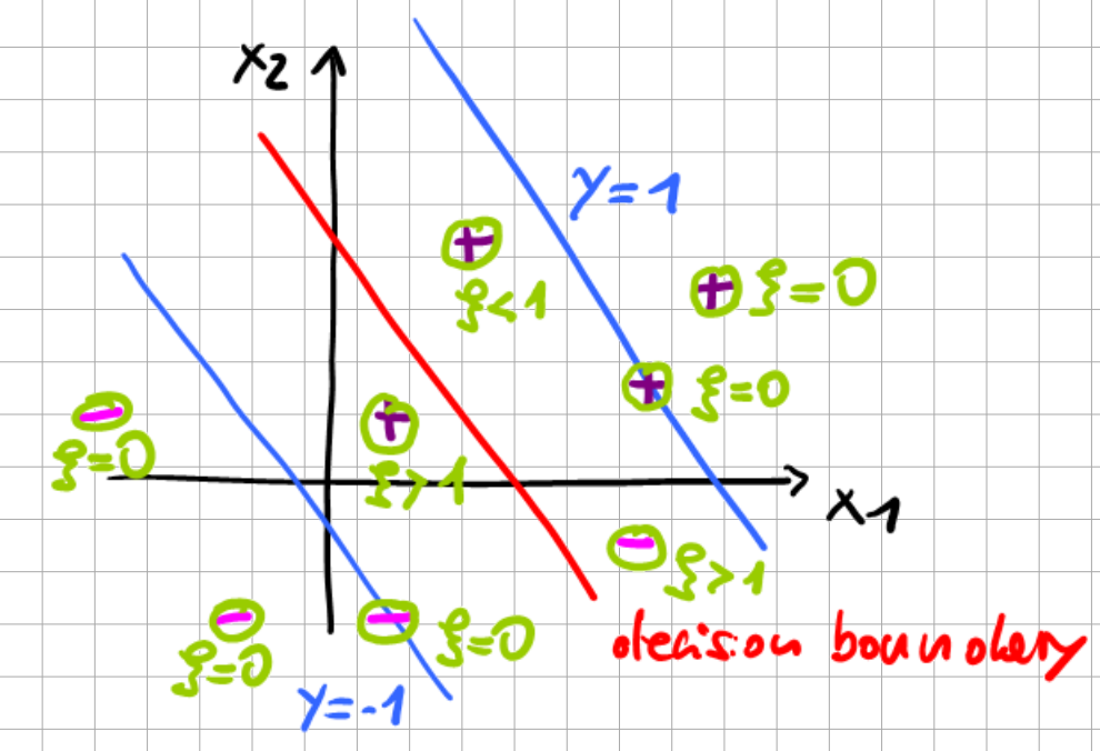
../_images/soft_margin_classifier.png — Fig. 6.9 Soft Margin Classifier.#

6.4. Advanced Topics: Sequential Minimal Optimization (SMO)#

Efficient algorithm for solving the SVM dual problem
Based on Coordinate Ascent algorithm.

6.4.1. Coordinate Ascent#

Task : find $max_{x} f (x_{1}, \dots, x_{m})$
Perform a component-wise search on $x$

Algorithm

do until converged
for $i = 1, \dots, m$
$x_{i}^{(k + 1)} = \underset{{\tilde{x}}_{i}}{argmax} f (x_{1}^{(k)}, \dots, {\tilde{x}}_{i}, \dots, x_{m}^{(k)})$
end for
end do

Sketch of algorithm

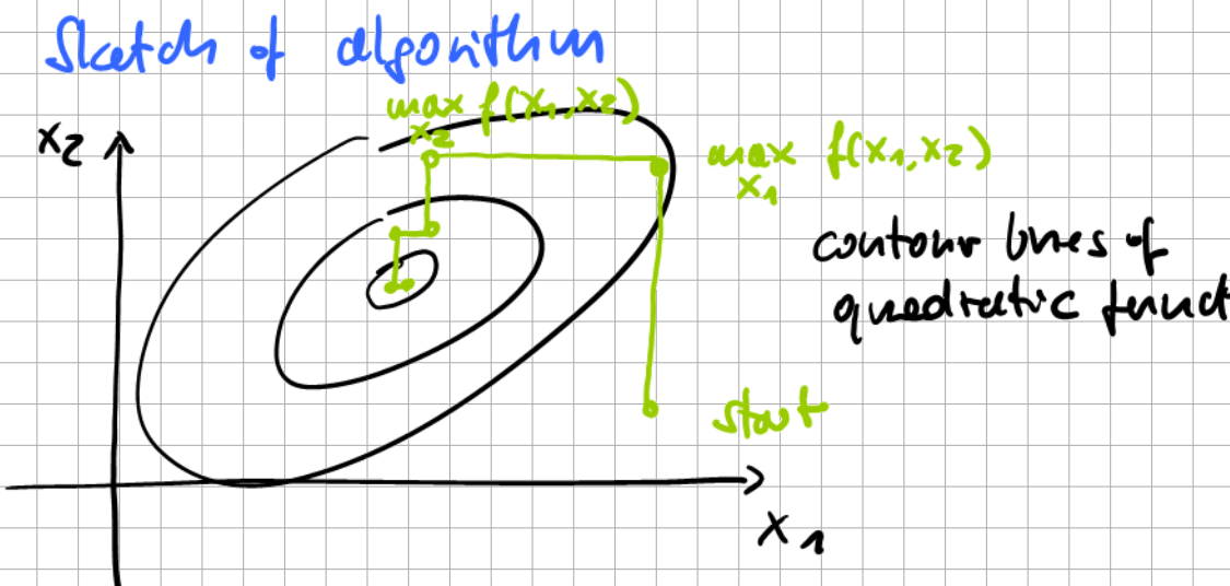
../_images/sequential_minimal_optimization.png — Fig. 6.10 Sequential Minimal Optimization.#

Coordinate ascent converges for convex continuous functions but may not converge to the dual optimum!

6.4.2. Outline of SMO for SVM#

Task: solve SVM dual optimization problem

(6.49)#

\begin{array}{r} \begin{aligned} max_{α} θ_{D} (α) & = max_{α} (\sum_{i = 1}^{m} α_{i} - \frac{1}{2} \sum_{i, j = 1}^{m} y^{(i)} y^{(j)} α_{i} α_{j} ⟨ x^{(i)}, x^{(j)} ⟩) \\ s.t. & {\begin{matrix} 0 \leq α_{i} \leq C, i = 1, \dots, m \\ \sum_{i = 1}^{m} α_{i} y^{(i)} = 0 \end{matrix} \end{aligned} \end{array}

Consider now an iterative update for finding the optimum:

Iteration step delivers a constraint satisfying set of $α_{i}$ .
Can we just change some $α_{j} ϵ$ { $α_{1}$ ,…., $α_{m}$ } according to coordinate ascent for finding the next iteration update?
- No, because $\sum_{i = 1}^{m} α_{i} y^{(i)} = 0$ constrains the sum of all $α_{i}$ , and varying only a single $α_{p}$ may lead to constraint violation
Fix it by changing a pair of $α_{p}, α_{q}$ , $p \neq q$ , simultaneously.

$\Rightarrow$ the SMO algorithm.

Algorithm

do until convergence criterion satisfied

Given $α^{(k)}$ constraint satisfying
Select $α_{p}^{(k + 1)} = α_{p}^{(k)}, α_{q}^{(k + 1)} = α_{q}^{(k)}$ for $p \neq q$ following some estimate which $p, q$ will give fastest ascent
Find $(α_{p}^{(k + 1)}, α_{q}^{(k + 1)}) = \underset{α_{p}, α_{q}}{argmax} θ_{D} (x_{1}^{(k)}, \dots, α_{p}, \dots, α_{q}, \dots, x_{m}^{(k)})$ // except for $α_{p}, α_{q}$ all others are kept fixed.

end do

Convergence criterion for SMO: check whether KKT conditions are satisfied up to a chosen tolerance.

Discussion of SMO

assume $α^{(k)}$ given with $\sum_{i = 1}^{m} y^{(i)} α_{i}^{(k)} = 0$
pick $α_{1} = α_{1}^{(k)}$ and $α_{2} = α_{2}^{(k)}$ for optimization

(6.50)#

\Rightarrow α_{1} y^{(1)} + α_{2} y^{(2)} = - \sum_{i = 3}^{m} α_{i} y^{(i)} = ρ

Note that the r.h.s. is constant during the current iteration step.

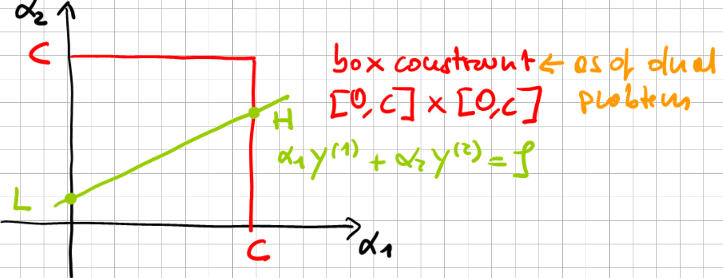
../_images/sequential_minimal_optimization_truncation.png — Fig. 6.11 Truncation during Sequential Minimal Optimization.#

The box constraints imply $L \leq α_{2} \leq H$ . Note that depending on the slope of the line, L or H may be clipped by the box constraint.

$α_{1} y^{(1)} + α_{2} y^{(2)} = ρ$

$\Rightarrow α_{1} = (ρ - α_{2} y^{(2)}) y^{(1)}$

$\to$ Do you see what happened here?

Answer:

$α_{1} y^{(1)} + α_{2} y^{(2)} = ρ / \cdot y^{(1)}$

$\Rightarrow α_{1} y^{(1)^{2}} = (ρ - α_{2} y^{(2)}) y^{(1)}$

$y^{(1)^{2}} = 1,$ as $y \in {- 1, 1}$

(6.51)#

\Rightarrow θ_{D} (α) = \sum_{i = 1}^{m} α_{i} - \frac{1}{2} \sum_{i, j = 1}^{m} y^{(i)} y^{(j)} α_{i} α_{j} ⟨ x^{(i)}, x^{(j)} ⟩

with $α_{1} = (ρ - α_{2} y^{(2)}) y^{(1)}$ thus becomes a quadratic function of $α_{2}$ , as all other $α_{j \neq 1, 2}$ are fixed.

$θ_{D} (α_{2}) = A α_{2}^{2} + B α_{2} + c o n s t .$ can be solved for $a r g max_{α_{2}} θ_{D} (α_{2}) = α_{2}^{^{'}}$
$α_{2}^{^{'}} \to$ box constraints $\to α_{2}^{^{″}}$

(6.52)#

\begin{array}{r} α_{2}^{^{″}} = {\begin{cases} H, α_{2}^{^{'}} > H \\ α_{2}^{^{'}}, L \leq α_{2}^{^{'}} \leq H \\ L, α_{2}^{^{'}} < L \end{cases} \end{array}

set $α_{2}^{(k + 1)} = α_{2}^{^{″}}$

(6.53)#

α_{1}^{(k + 1)} = (ρ - α_{2}^{(k + 1)} y^{(2)}) y^{(1)}

next iteration update

6.5. Kernel Methods#

Consider binary classification in the non-linearly-separable case, assuming that there is a feature map $φ (x) \in R^{n}$ transforming the input $x \in R^{d}$ to a space which is linearly separable.

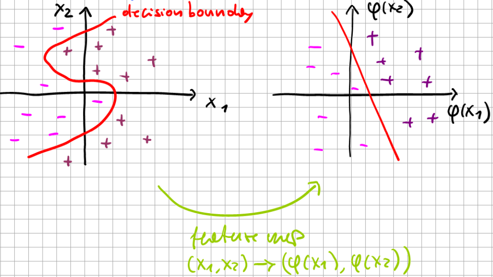
../_images/kernel_feature_map.png — Fig. 6.12 Feature map transformation.#

The feature map is essentially a change of basis as:

(6.54)#

x \to φ (x)

In general, $x$ and $φ$ are vectors where $φ$ has the entire $x$ as an argument. The resulting modified classifier becomes

(6.55)#

h (x) = g (ω^{T} φ (x) + b) .

Example: XNOR

The following classification problem is non-linear, as there is no linear decision boundary.

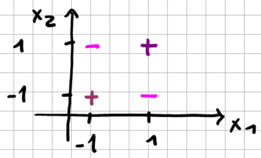
../_images/xnor_example.png — Fig. 6.13 XNOR example.#

Upon defining a feature map $φ (x_{1}, x_{2}) = x_{1} x_{2}$ (maps 2D $\to$ 1D), we get

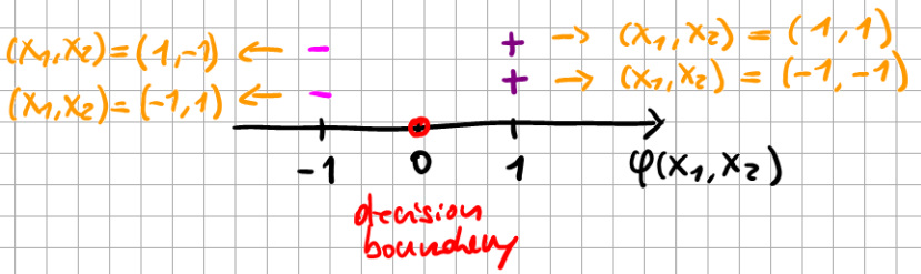
../_images/xnor_example_embedded.png — Fig. 6.14 XNOR after feature mapping.#

Example: Circular Region

Given is a set of points $x \in R^{2}$ with two possible labels: purple ( $- 1$ ) and orange ( $1$ ), as can be seen in the left figure below. The task is to find a feature map such that a linear classifier can perfectly separate the two sets.

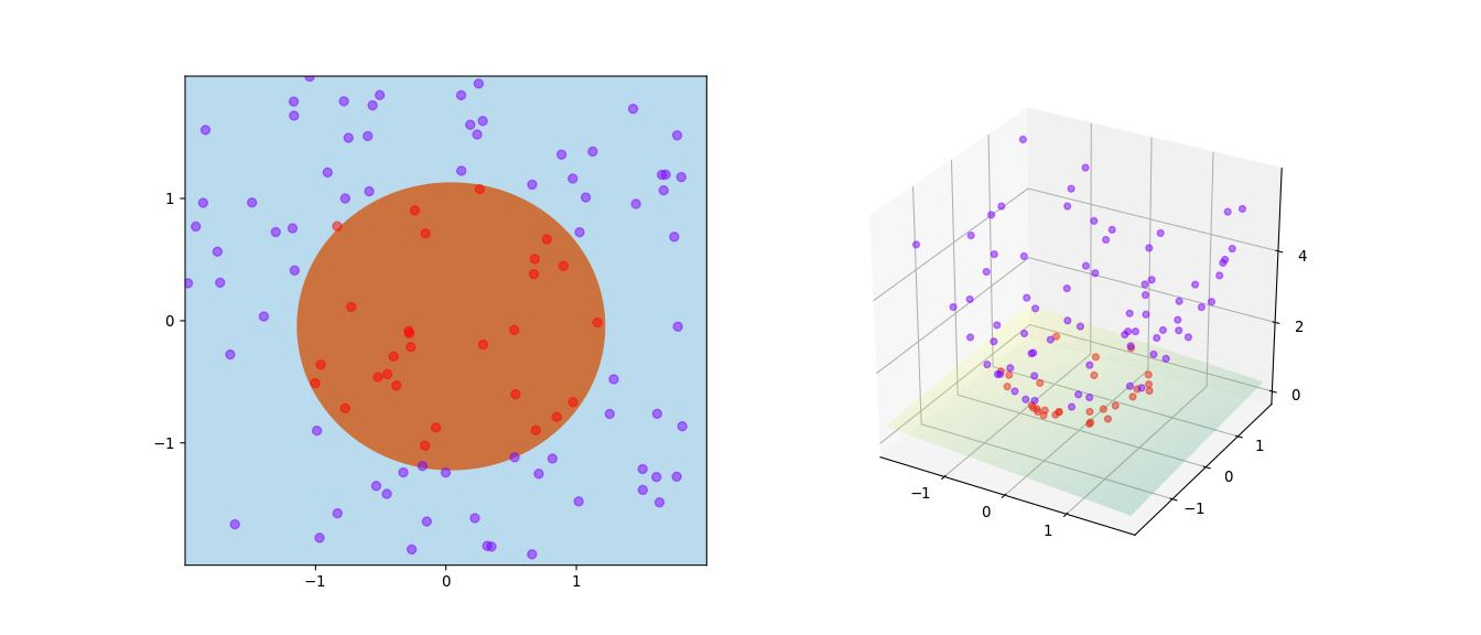
../_images/kernel_trick_idea.png — Fig. 6.15 Binary classification of a circular region (Source: Wikipedia).#

Here, it is again obvious that if we embed the inputs in a 3D space by adding their squares, i.e., $φ ((x_{1}, x_{2})) = (x_{1}, x_{2}, x_{1}^{2} + x_{2}^{2})$ , we will be able to draw a hyperplane separating the subsets.

But of course, these examples are constructed, as here we could immediately guess $φ (x_{1}, x_{2})$ . In general, this is not possible.

Recall: the dual problem of SVM involves a scalar product $x^{(i) ⊤} x^{(j)}$ of feature vectors. $\Rightarrow$ motivates the general notation of a dual problem with feature maps.

6.5.1. Dual representations#

Motivated by Least Mean Squares (LMS) regression, we consider the following regularized cost function:

(6.56)#

J (ω) = \sum_{i = 1}^{m} {(w^{T} φ (x^{(i)}) - y^{(i)})}^{2} + \frac{λ}{2} ω^{T} ω,

with penalty parameter $λ ⩾ 0$ .

Regularization helps to suppress the overfitting problem (see Tricks of Optimization). The squared L2 regularization above is also called Tikhonov regularization. In machine learning, linear regression in combination with Tikhonov regularization is often dubbed ridge regression.

Setting the gradient of that loss to zero $\nabla_{ω} J = 0$ we obtain the solution

(6.57)#

ω = - \frac{1}{λ} \sum_{i = 1}^{m} (w^{T} φ (x^{(i)}) - y^{(i)}) φ (x^{(i)}) = Φ^{T} a,

with design matrix $Φ$ using the feature map $φ$ defined as

(6.58)#

\begin{array}{r} Φ = [\begin{array}{c} ⋮ \\ φ (x^{(i)}) \\ ⋮ \end{array}] \in R^{m \times n} \end{array}

and

(6.59)#

\begin{array}{r} a = - \frac{1}{λ} [\begin{array}{c} ⋮ \\ w^{T} φ (x^{(i)}) - y^{(i)} \\ ⋮ \end{array}] \in R^{m} . \end{array}

Substituting the necessary condition $ω = Φ^{T} a$ into $J (ω)$ we obtain the dual problem:

(6.60)#

\begin{array}{r} \begin{aligned} J_{D} (a) = & \frac{1}{2} a^{T} Φ Φ^{T} Φ Φ^{T} a - a^{T} Φ Φ^{T} y + \frac{1}{2} y^{T} y + \frac{λ}{2} a^{T} Φ Φ^{T} a \\ = & \frac{1}{2} a^{T} K K a - a^{T} K y + \frac{1}{2} y^{T} y + \frac{λ}{2} a^{T} K a \end{aligned} \end{array}

Here, $K = Φ Φ^{T}$ is a Grammatrix generated by a vector $φ$ according to $K_{i j} = ⟨ φ_{i}, φ_{j} ⟩$ where $⟨ \cdot, \cdot ⟩$ is an inner product - here $⟨ φ (x^{(i)}), φ (x^{(j)}) ⟩$ .

(6.61)#

K_{i j} = φ^{T} (x^{(i)}) φ (x^{(j)}) =: K (x^{(i)}, x^{(j)}),

where $K (x^{(i)}, x^{(j)})$ is the kernel function.

Now we find that we can express the LMS prediction in terms of the kernel function:

(6.62)#

J_{D} (a) = \frac{1}{2} a^{T} K K a - a^{T} K y + \frac{1}{2} y^{T} y + \frac{λ}{2} a^{T} K a .

In order to find $max_{a} J_{D} (a)$ we set $\nabla_{a} J_{D} (a) = 0$ .

(6.63)#

\begin{array}{r} \begin{aligned} \Rightarrow K a - y + λ I a = 0 \\ \Rightarrow a = (K + λ I)^{- 1} y \end{aligned} \end{array}

Upon inserting this result into a linear regression model with feature mapping

(6.64)#

\begin{array}{r} \begin{aligned} h (x) & = ω^{T} φ (x) + b = a^{T} Φ φ (x) = Φ^{T} φ (x) a \\ = k^{T} (K + λ I)^{- 1} y, \end{aligned} \end{array}

where $k_{i} = K (x^{(i)}, x)$ are the components of K.

The kernel trick refers to this formulation of the learning problem, which relies on computing the kernel similarities between a pair of input points $x$ and $x^{'}$ , instead of computing $φ (x)$ explicitly.

The term Support Vector Machine typically refers to a margin classifier using the kernel formulation.

Now, let’s do some bookkeeping using the number of data points $M$ and the dimension of the input data $N$ .

(6.65)#

\underset{M}{\underset{⏟}{a}} = \underset{M \times M}{\underset{⏟}{(K - λ I)^{- 1}}} \underset{M}{\underset{⏟}{y}} .

Recall from the lecture on linear models that $\underset{N}{\underset{⏟}{ϑ}} = \underset{N \times N}{\underset{⏟}{(X^{T} X)^{- 1}}} \underset{N \times M}{\underset{⏟}{X^{T}}} \underset{M}{\underset{⏟}{y}}$

As typically $M >> N$ we see that solving the dual problem for LMS requires us to invert a $M \times M$ matrix, whereas the primal problem tends only to a $N \times N$ matrix.

The benefit of the dual problem with the kernel $K (x, x^{'})$ is that now we can work with the kernel directly $\Rightarrow$ dimensionality of $φ (x)$ matters no longer. $\Rightarrow$ we can consider even an infinite-dimensional feature vector $N \to \infty$ , i.e. a continuous $φ (x)$

6.5.2. Construction of suitable kernels#

construction from the feature map

(6.66)# $K (x, x^{'}) = φ^{T} (x) φ (x^{'}) = \sum_{i = 1}^{N} φ_{i} (x) φ_{i} (x^{'})$
direct construction with the constraint that a valid kernel is obtained, i.e., it actually needs to correspond to a possible feature map scalar product.

A necessary and sufficient condition for a valid kernel is that $K$ is positive semidefinite for all $x$ .

Example: Kernel 1

Given is $x, x^{'} \in R^{N}$ and a scalar kernel

(6.67)#

\begin{array}{r} \begin{aligned} K (x, x^{'}) & = (x^{T} x^{'})^{2} \\ = \sum_{i = 1}^{N} x_{i} x_{i}^{'} \sum_{j = 1}^{N} x_{j} x_{j}^{'} \\ = \sum_{i} \sum_{j} x_{i} x_{j} x_{i}^{'} x_{j}^{'} . \end{aligned} \end{array}

The corresponding feature map for $K (x, x^{'}) = φ^{T} (x) φ (x^{'})$ and with $N = 3$ is

(6.68)#

\begin{array}{r} φ (x) = [\begin{array}{l} x_{1} x_{1} \\ x_{1} x_{2} \\ x_{1} x_{3} \\ x_{2} x_{1} \\ \dots \\ x_{3} x_{3} \end{array}] \end{array}

Example: Kernel 2

Alternative kernel with parameter $c$ :

(6.69)#

K (x, x^{'}) = (x^{T} x^{'} + c)^{2} = \sum_{i, j} x_{i} x_{j} x_{i}^{'} x_{j}^{'} + \sum_{i} \sqrt{2 c} x_{i} \sqrt{2 c} x_{j} + c^{2}

belongs to

(6.70)#

\begin{array}{r} φ (x) = [\begin{array}{l} x_{1} x_{1} \\ x_{1} x_{2} \\ \dots \\ x_{3} x_{3} \\ \sqrt{2 c} x_{1} \\ \sqrt{2 c} x_{2} \\ \sqrt{2 c} x_{3} \\ c \end{array}] \end{array}

Considering that $φ (x)$ and $φ (x^{'})$ are vectors, the scalar product $K (x, x^{'}) = φ^{T} (x) φ (x^{'})$ expresses the projection of $φ (x^{'})$ onto $φ (x)$ .

$\Rightarrow$ The larger the kernel value, the more parallel the vectors are. Conversely, the smaller, the more orthogonal they are.

$\Rightarrow$ Intuitively $K (x, x^{'})$ is a measure of “how close” $φ (x)$ and $φ (x^{'})$ are.

Example: Gaussian kernel

(6.71)#

\begin{array}{r} K (x, x^{'}) = \exp {- \frac{(x - x^{'})^{T} (x - x^{'})}{2 σ^{2}}} \\ {\begin{cases} \approx 1, x and x^{'} close \\ \approx 0, x and x^{'} far apart \end{cases} \end{array}

Now, we illustrate that a valid kernel is positive semidefinite, which is the above-mentioned necessary condition.

6.5.2.1. Proof:#

(6.72)#

K_{i j} = φ^{T} (x^{(i)}) φ (x^{(j)}) = φ^{T} (x^{(j)}) φ (x^{(i)}) = K_{j i}

(6.73)#

\begin{array}{r} \begin{aligned} \Rightarrow (x^{'})^{T} K x^{'} & = x_{i}^{'} K_{i j} x_{j}^{'} \\ = x_{i}^{'} φ^{T} (x^{(i)}) φ (x^{(j)}) x_{j}^{'} \\ = x_{i}^{'} φ_{k}^{(i)} φ_{k}^{(j)} x_{j}^{'} \\ = \sum_{k} (x_{i}^{(i)} φ_{k}^{(i)})^{2} ⩾ 0 \end{aligned} \end{array}

The necessary and sufficient condition is due to Mercer’s theorem:

A given $K : R^{N} \times R^{N} \to R$ is a valid kernel if for any { $x^{(1)}, . . ., x^{(m)}$ }, $m < \infty$ the resulting $K$ is positive semidefinite (which implies that it also must be symmetric). We can still apply MMC or slack-variable SMC for non-separable sets: We simply replace the feature-scalar product within the SVM prediction.

(6.74)#

h (x) = ω^{* T} x + b^{*} = \sum_{i = 1}^{m} α_{i}^{*} y^{(i)} ⟨ x^{(i)}, x ⟩ + b^{*}

We replace $⟨ x^{(i)}, x ⟩$ by $k (x^{(i)}, x)$ .

(6.75)#

h (x) = \sum_{i = 1}^{m} α_{i}^{*} y^{(i)} k (x^{(i)}, x) + b^{*}

This pulls through into the dual problem for determining $α_{i}^{*}$ and $b^{*}$ such that by picking a suitable kernel function, we may get close to a linearly separable transformation function without actually performing the feature mapping.

6.6. Recapitulation of SVMs#

Problem of non-linearly separable sets
- Introduction of controlled violations of the strict margin constraints
- Introduction of feature maps
Controlled violation: slack variables $\to l_{1}$ -regularized opt. problem $\to$ modified dual problem $\to$ solution by SMO
Feature map: kernel function (tensorial product of feature maps) $\to$ reformulated dual optimization problem $\to$ prediction depends only on the kernel function
Kernel construction: a lot of freedom but $\to$ valid kernel
Important kernel: Gaussian
Solution of non-separable problems:
- Pick a suitable kernel function
- Run SVM with a kernel function

6.7. Further References#

[Ng, 2022], Chapters 5 and 6
[Murphy, 2022], Section 17.3
[Bishop, 2006], Appendix E: Lagrange Multipliers