8. Gradients#
Learning outcome
How does automatic differentiation (AD) work?
What is the difference between forward-mode and reverse-mode AD?
How to construct the compute graph for backpropagation?
Gradients are a general tool of utility across many scientific domains and keep reappearing across areas. Machine learning is just one of a much larger group of examples that utilizes gradients to accelerate its optimization processes. Breaking the uses down into a few rough areas, we have:
Machine learning (Backpropagation, Bayesian Inference, Uncertainty Quantification, Optimization)
Scientific Computing (Modeling, Simulation)
But what are the general trends driving the continued use of automatic differentiation as compared to finite differences or manual adjoints?
The writing of manual derivative functions becomes intractable for large codebases or dynamically generated programs
We want to be able to automatically generate our derivatives
8.1. A Brief Incomplete History#
1980s/1990s: Automatic Differentiation in Scientific Computing mostly spearheaded by Griewank, Walther, and Pearlmutter
Adifor
Adol-C
…
2000s: Rise of Python begins
2015: Autograd for the automatic differentiation of Python & NumPy is released
2016/2017: PyTorch & Tensorflow/JAX are introduced with automatic differentiation at their core. See this Tweet for the history of PyTorch and its connection to JAX.
2018: JAX is introduced with its very thin Python layer on top of TensorFlow’s compilation stack, where it performs automatic differentiation on the highest representation level
2020-2022: Forward-mode estimators to replace the costly and difficult-to-implement backpropagation are being introduced
With the cost of machine learning training dominating data center bills for many companies and startups alike, there exist many alternative approaches out there to replace gradients, but none of them have gained significant traction so far. But it is definitely an area to keep an eye out for.
8.2. The tl;dr of Gradients#
We give a brief overview of the two modes, with derivations of the properties as well as examples following later.
8.2.1. Forward-Mode Differentiation#
Examining a classical derivative computation
Then, in the case of the forward-mode derivative, the gradient is evaluated from the right to the left. The Jacobian of the intermediate values is then accumulated with respect to the input \(x\)
and the information flows in the same direction as the computation. This means that we do not require any elaborate caching system to hold values in memory for later use in the computation of a gradient, and hence require much less memory and are left with a much simpler algorithm.
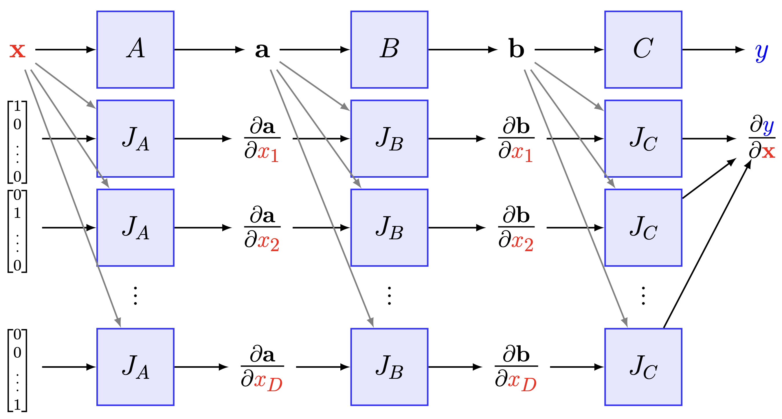
Fig. 8.1 Forward-mode differentiation. (Source: [Maclaurin, 2016], Section 2)#
8.2.2. Reverse-Mode Differentiation (Backpropagation)#
Taking a typical case of reverse-mode differentiation, or as it is called in machine learning, “backpropagation”
In the case of reverse-mode differentiation, the evaluation of the gradient is then performed from the left to the right. The Jacobians of the output \(y\) are then accumulated with respect to each of the intermediate variables
and the information flows in the opposite direction of the function evaluation, which points to the main difficulty of reverse-mode differentiation. We require an elaborate caching system to hold values in memory for when they are needed for the gradient computation, and hence require much more memory and are left with a much more difficult algorithm.
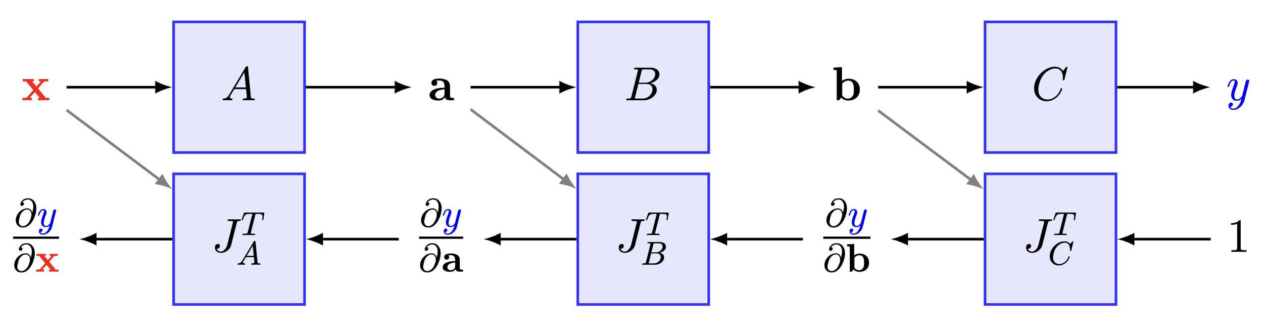
Fig. 8.2 Reverse-mode differentiation. (Source: [Maclaurin, 2016], Section 2)#
Example: AD on a Linear Model
Given is the linear model \(h(x)=w \cdot x+b\) that maps from the input \(x\in \mathbb{R}\) to the output \(y\in \mathbb{R}\), as well as a dataset of a single measurement pair \(\{(x=1, y=7)\}\). The initial model parameters are \(w=2, b=3\). Compute the gradient of the MSE loss w.r.t. the model parameters, and run one step of gradient descent with step size \(0.1\). Draw all intermediate values in the provided compute graph below.
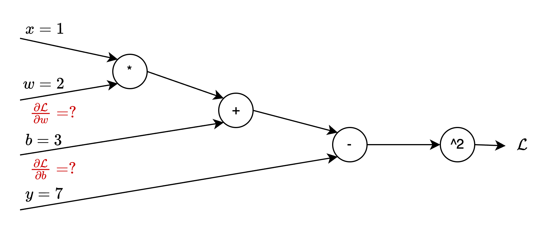
Fig. 8.3 AD example.#
Solution: Given that the loss function is scalar-valued, while the parameter space (\(w,b\)) is two-dimensional, we evaluate the gradients using reverse-mode AD. We first name and evaluate all intermediate values in the forward pass, denoted with black color in Fig. 8.4.
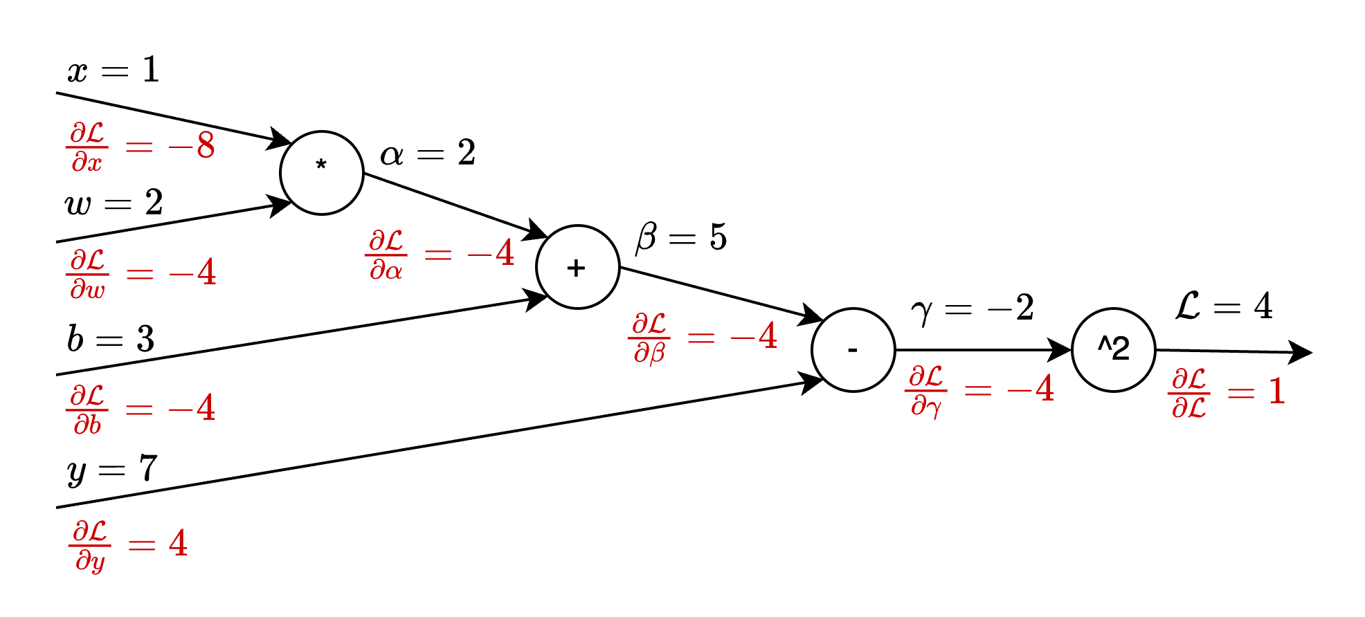
Fig. 8.4 AD example, solution.#
Then, we compute the gradients starting from the loss and then going backward, denoted in red in the figure.
Finally, one step of gradient descent results in the following update.
8.2.3. Forward- vs. Reverse-Mode#
The performance comparison between forward-mode and reverse-mode gradients can be broken down depending on the size of our input vector and our output vector. So for the case of abstracting our neural network as a function that takes an input vector of a certain size \(n\) and generates an output vector of a certain size \(m\)
Forward-mode: More efficient for gradients of scalar-to-vector functions, i.e. \(m >> n\)
Reverse-mode: More efficient for gradients of vector-to-scalar functions, i.e. \(m << n\)
As most loss functions in machine learning output a scalar value, reverse-mode differentiation is a very natural choice for these computations. A way to circumvent these issues of forward-mode differentiation and simplify the technical infrastructure in the background is to compose forward-mode with vectorization or only compute an estimator of the gradient where multiple forward-mode samples are used.
8.3. In-Depth Look#
We decompose the function \(f\) as
where we are essentially converting from space to space with each function. Each function is an abstraction for an individual neural network layer, as we will see in much more depth when constructing neural networks in the upcoming lectures or in the exercises later on.
where our overall network \(o = f(x)\) is broken down as
Using the chain rule we can then compute the Jacobian \(J_{f}(x) = \frac{\partial o}{\partial x}\) as
This approach to the computation would be highly inefficient. As such we rely on matrix computation for more efficiency, i.e.
In practice, we would love to have access to this Jacobian, but the reality is that in 99.99% of the cases, it is too expensive to compute, and as such, we have to make do with snippets from this Jacobian, namely the Jacobian Vector Product (JVP), and the Vector Jacobian Product (VJP).
The \(i\)-th row of \(J_{f}(x)\) gives us the vector Jacobian product (reverse-mode differentiation)
The \(j\)-th column of \(J_{f}(x)\) gives us the Jacobian vector product (forward-mode differentiation)
Examining the case for when \(n<m\), then it is more efficient to compute each column using the Jacobian vector product in a right-to-left manner, i.e., the right multiplication of a column vector gives us
which is then computed with forward-mode differentiation. The pseudoalgorithm is given below.
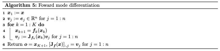
Fig. 8.5 Forward-mode algorithm.#
Returning to the cost advantage of forward-mode differentiation, in this specific case, the computation cost is \(\mathcal{O}(n)\). If we now have the case where \(n>m\), then it is more efficient to compute \(J_{f}(x)\) for each row using the vector Jacobian product (VJP) in a left-to-right manner, i.e.
for the solving of which reverse-mode differentiation is the most well-suited. The pseudo algorithm for which can be found below. The cost of computation in this case is \(\mathcal{O}(m)\).
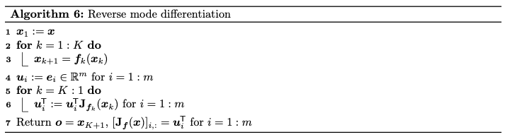
Fig. 8.6 Reverse-mode algorithm.#
8.4. A Practical Example#
Considering a simple feed-forward model with 4 layers, we now have the following computation setup represented as a directed acyclic graph:
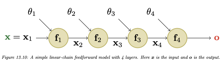
Fig. 8.7 Compute graph of a 4-layer feed-forward network.#
The MLP with one hidden layer is written down as
which is then represented as the following feedforward model:
The \(\theta_{k}\) are the optional parameters for each layer. As, by construction, the final layer returns a scalar, it is much more efficient to use reverse-mode differentiation to compute the gradient vectors in this case. We begin by computing the gradients of the loss with respect to the parameters in the earlier layers
This recursive computation procedure can subsequently be condensed down to a pseudo algorithm:
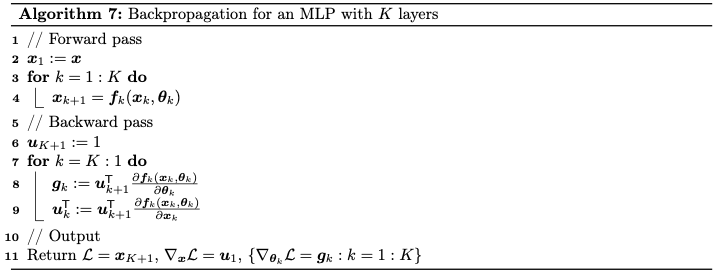
Fig. 8.8 Reverse-mode differentiation through an MLP.#
What is missing from this pseudo algorithm is the definition of the vector Jacobian product of each layer, which depends on the type and function of each layer. Or, in a slightly more intricate case, please see the example below for what this computation looks like in the case of backpropagation.
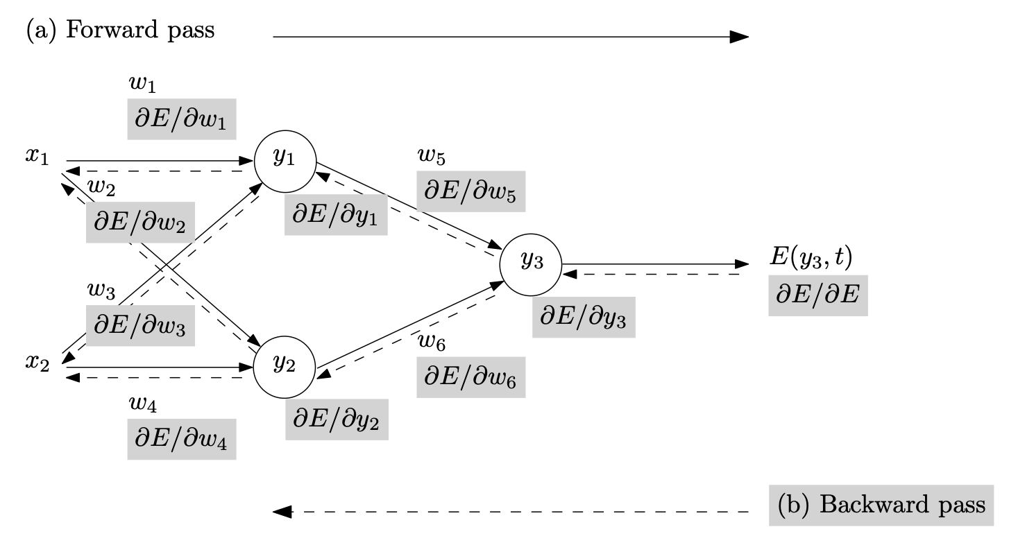
Fig. 8.9 More detailed compute graph of a feed-forward network (Source: [Baydin et al., 2018]).#
8.5. What are the Core-Levers of the Alternative Approaches#
Do we actually need accurate gradients for the training, or can we actually get away with much, much coarser gradients to power our training?
Approximate the reverse-mode gradients with the construction of cheap forward-mode gradients
By construction of a Monte-Carlo estimator for the reverse-mode gradient using forward-mode gradient samples
Randomizing the forward-mode gradients and then constructing an estimator
Taking gradients at different program abstraction levels. Taking the example of JAX, we have access to the following main program abstraction levels at which gradients can be computed
Python frontend
Jaxpr
MHLO
XLA
8.6. Further References#
Needs to be refactored
I2DL lecture by Matthias Niessner - Lecture on Backpropagation
Jax’s Autodiff Cookbook - a playful introduction to gradients
[Maclaurin, 2016] - Chapter 4 of Dougal MacLaurin’s PhD Thesis
Tangent: Automatic Differentiation Using Source Code Transformation in Python