9. Multilayer Perceptron#
Learning outcome
Write down the perceptron equation.
Name two popular nonlinear activation functions.
How does the Universal Approximation Theorem contradict empirical knowledge?
9.1. Limitations of Linear Regression#
Going back to lecture Tricks of Optimization, we discussed that the most general linear model could be any linear combination of \(x\)-values lifted to a predefined basis space \(\varphi(x)\), e.g., polynomial, exponent, sin, tanh, etc. basis:
We also saw that through hyperparameter tuning, one can find a basis that captures the underlying true relation between inputs and outputs well. In fact, for many practical problems, the approach of manually selecting meaningful basis functions and then training a linear model will be good enough, especially if we know something about the data beforehand.
The problem is that for many tasks, we don’t have such a-priori information, and exploring the space of all possible combinations of basis functions ends in an infeasible combinatoric problem. Especially if our datasets are large, e.g., ImageNet, it is unrealistic to think that we can manually transform the inputs to a linearly separable space.
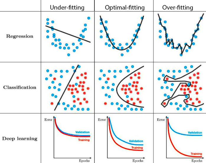
Fig. 9.1 Under- and overfitting (Source: Techniques for handling underfitting and overfitting in Machine Learning)#
Q: If linear models are not all, what else?
Deep Learning is the field that tries to systematically explore the space of possible non-linear relations \(h\) between input \(x\) and output \(y\). As a reminder, a non-linear relation can be, for example
In the scope of this class, we will look at the most popular and successful non-linear building blocks. We will see the Multilayer Perceptron, Convolutional Layer, and Recurrent Neural Network.
9.2. Perceptron#
Perceptron is a binary linear classifier and a single-layer neural network.
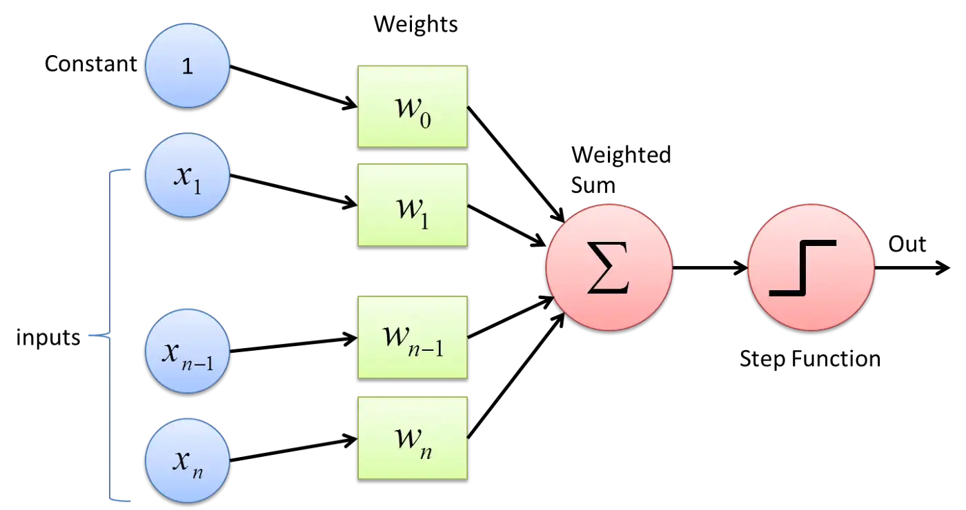
Fig. 9.2 The perceptron (Source: What the Hell is Perceptron?)#
The perceptron generalizes the linear hypothesis \(\vartheta^{\top} x\) by subjecting it to a step function \(f\) as
Note: The term \(\vartheta x\) is actually an affine transformation, not just linear. We use the notation with \(w_0 = b\) for brevity.
In the case of two-class classification, we use the sign function
\(f(a)\) is called activation function as it represents a simple model of how neurons respond to input stimuli. Other common activation functions are the sigmoid, tanh, and ReLU (\(=\max(0,x)\)).
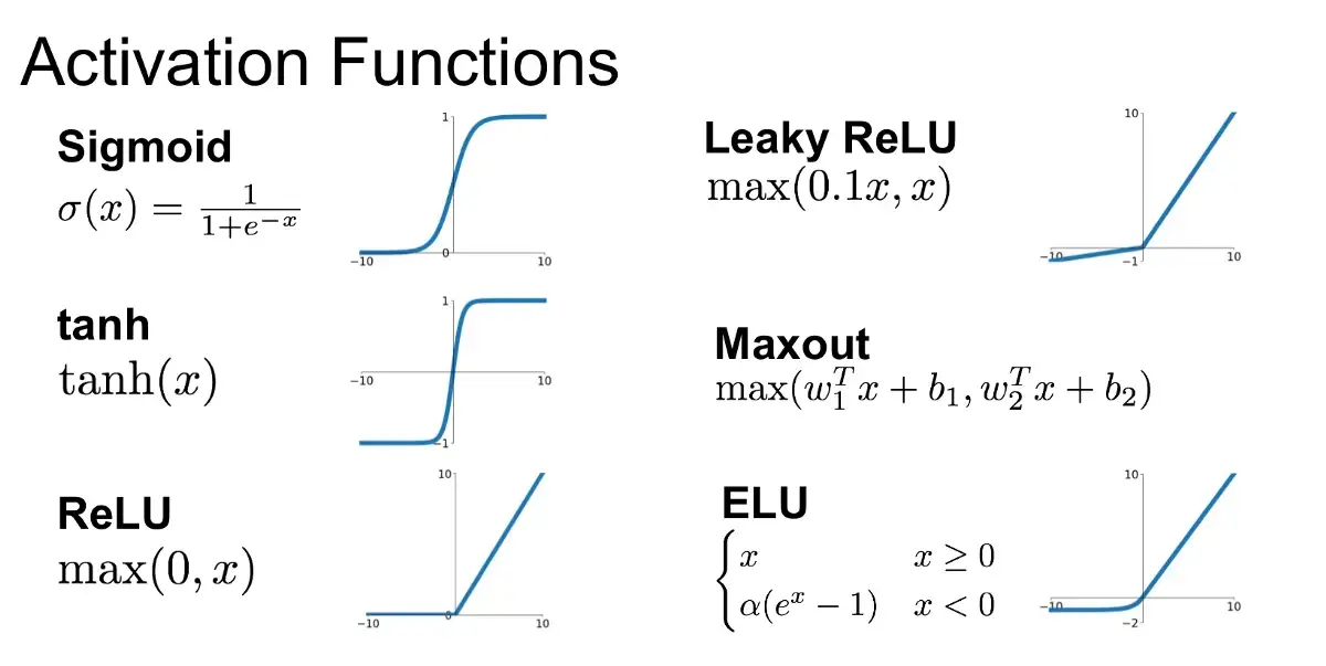
Fig. 9.3 Activation functions (Source: Introduction to Different Activation Functions for Deep Learning)#
9.3. Multilayer Perceptron (MLP)#
If we stack multiple perceptrons after each other with a user-defined dimension of the intermediate (a.k.a. latent or hidden) space, we get a multilayer perceptron.
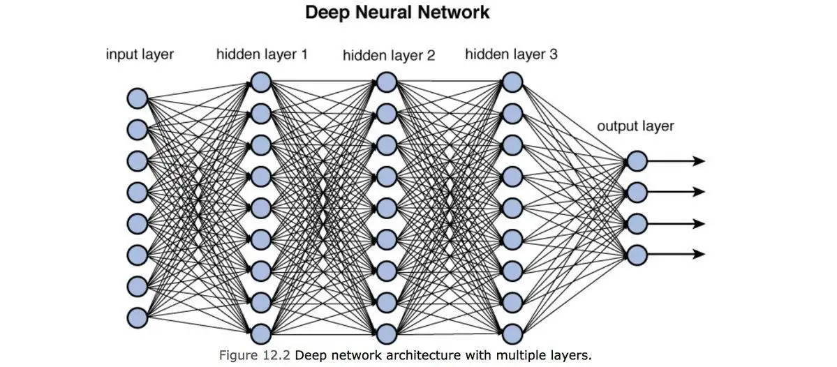
Fig. 9.4 Multilayer Perceptron (Source: Training Deep Neural Networks)#
We could write down the stack of such layer-to-layer transformations as
In the image above, the black line connecting entry \(i\) of the input with the corresponding entry \(j\) of hidden layer 1 corresponds to the row \(i\) and column \(j\) of the learnable weights matrix \(W_{1}\). Note that the output layer does not have an activation function - in the case of regression, we typically stop with the linear transformation, and in the case of classification, we typically apply the softmax function to the output vector.
It is crucial to have non-linear activation functions. Why? Simply concatenating linear functions results in a new linear function! You immediately see it if you remove the activations \(f_i\) in the equation above.
By the Universal Approximation Theorem, a single-layer perceptron with any “squashing” activation function (i.e., \(h(x)=W_2 f(W_1 x)\)) can approximate essentially any functional \(h: x \to y\). More on that in [Goodfellow et al., 2016], Section 6.4.1. However, empirically we see improved performance when we stack multiple layers, adding the depth (number of hidden layers) and width (dimension of hidden layers) of a neural network to the hyperparameters of paramount importance.
Exercise: Learning XOR
Find the simplest MLP capable of learning the XOR function, and fit its parameters.
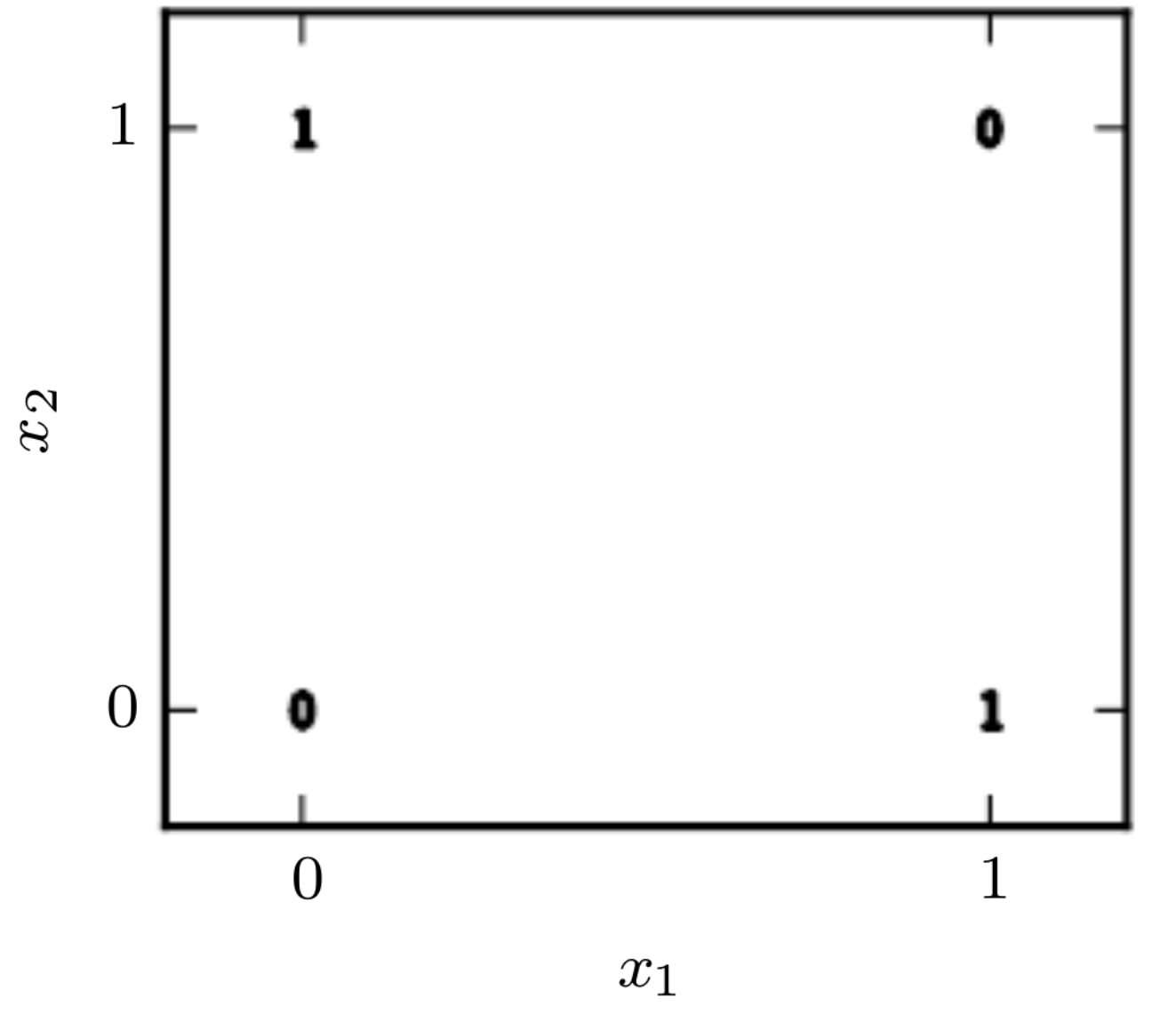
Fig. 9.5 XOR function (Source: [Goodfellow et al., 2016], Section 6.1)#
9.4. Further References#
[Goodfellow et al., 2016], Chapter 6