Introduction#
Famous Recent Examples of Scientific Machine Learning#
With scientific machine learning becoming an ever more prominent mainstay at machine learning conferences, and ever more venues and research centers at the intersection of machine learning and the natural sciences/engineering appearing there exist ever more impressive examples of algorithms that connect the very best of machine learning with deep scientific insight into the respective underlying problem to advance the field.
Below are a few prime examples of recent flagship algorithms in scientific machine learning, every single one of which personifies the very best algorithmic approaches we have available to us today.
AlphaFold - predicts 3D protein structure given its sequence:#
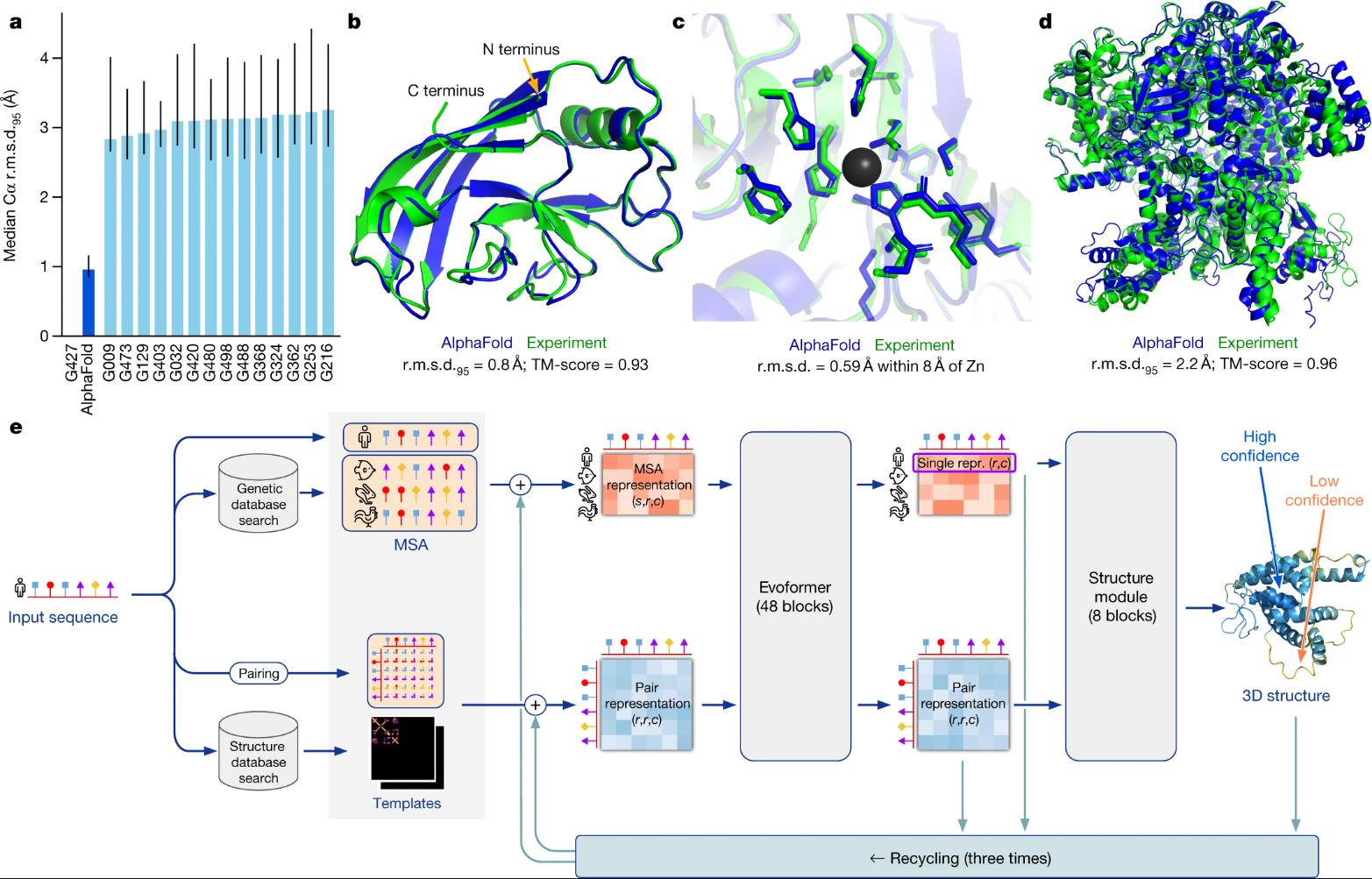
Fig. 1 AlphaFold model. (Source: Jumper et al., 2021)#

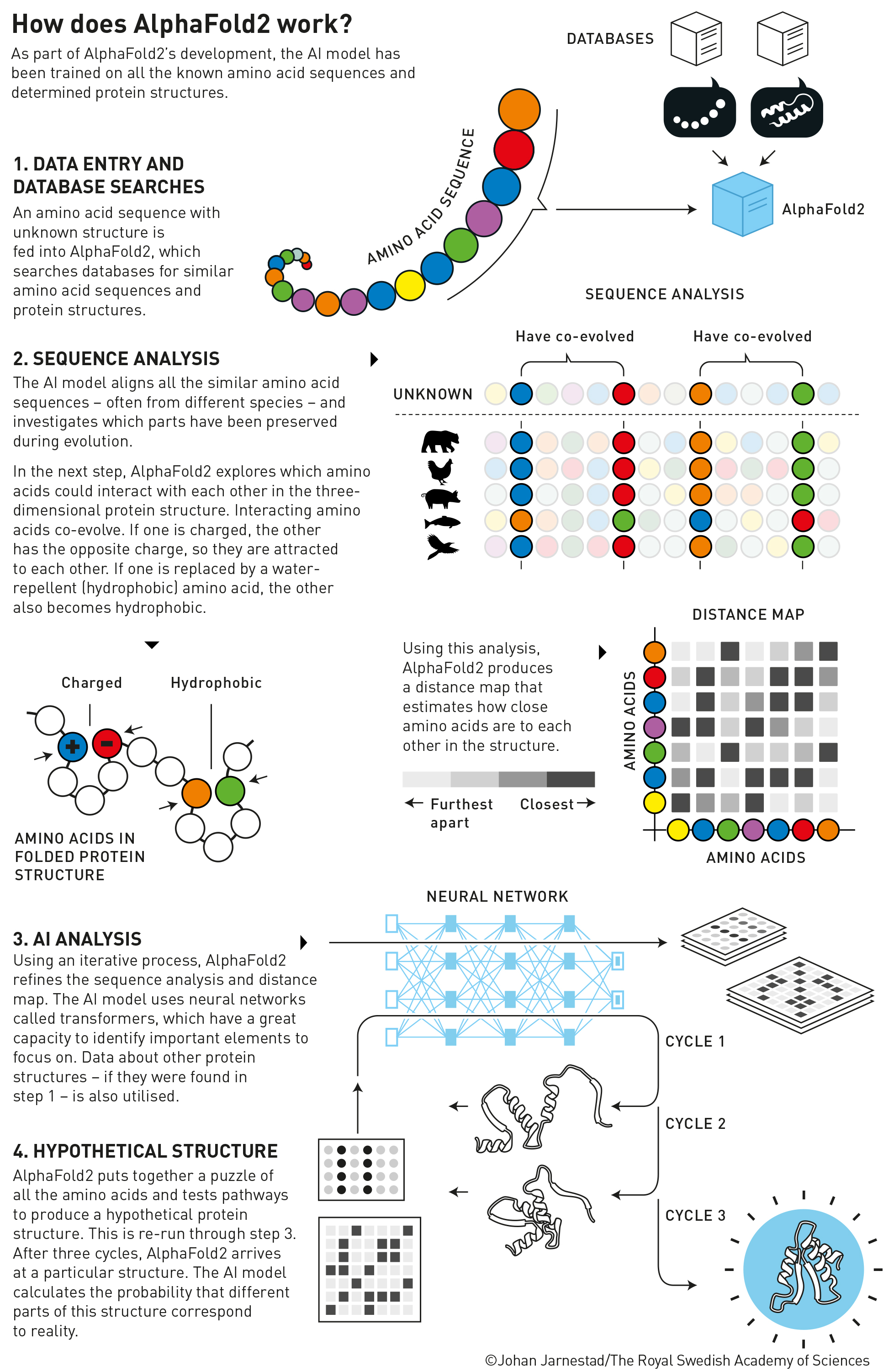
Fig. 3 How does AlphaFold2 work? (Source: nobelprize.org)#
GNS - capable of simulating the motion of water particles:#
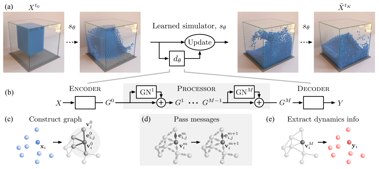
Fig. 4 GNS model. (Source: Sanchez-Gonzalez et al., 2020)#
Codex - translating natural language to code:#
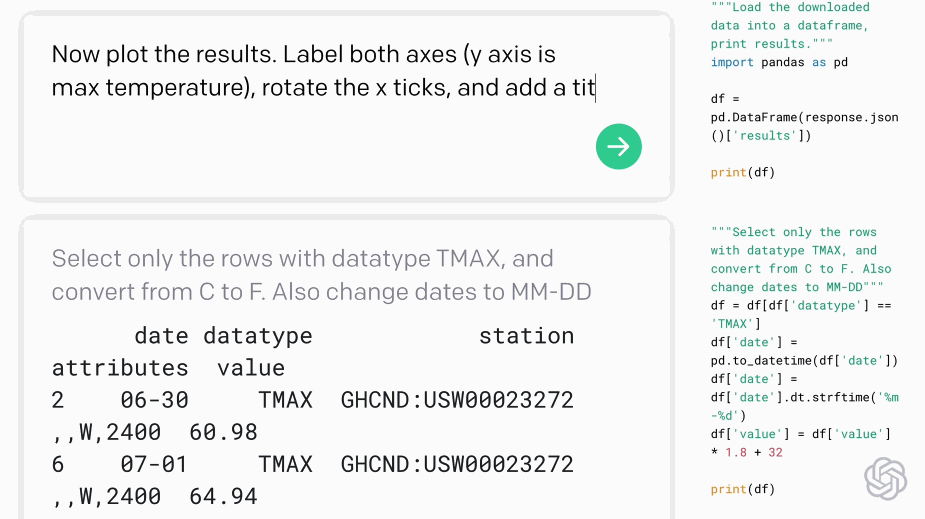
Fig. 5 Codex demo (Source: openai.com)#
Geometric Deep Learning#
Geometric deep learning aims to generalize neural network models to non-Euclidean domains such as graphs and manifolds. Good examples of this line of research include:
SFCNN - steerable rotation equivariant CNN, e.g. for image segmentation#
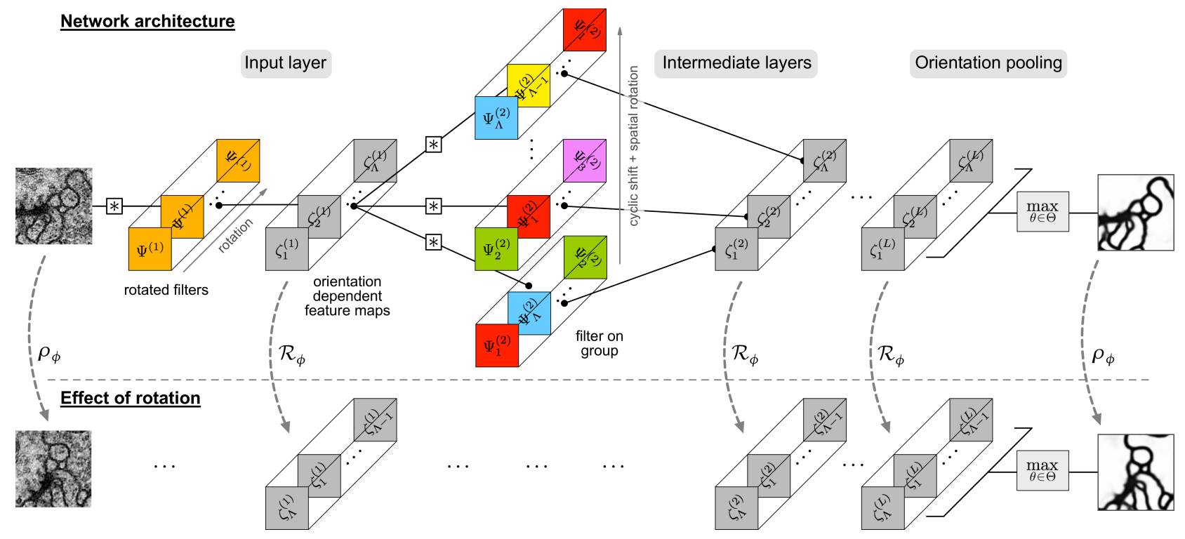
Fig. 6 SFCNN model. (Source: Weiler et al., 2018)#
SEGNN - molecular property prediction model#
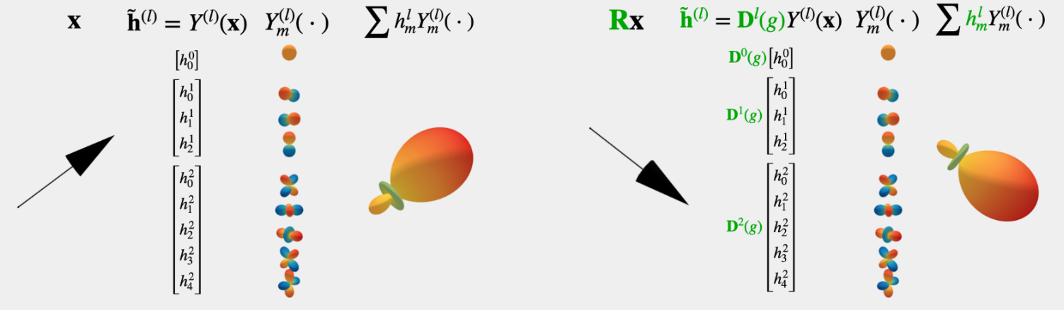
Fig. 7 SEGNN model. (Source: Brandstetter et al., 2022)#
Stable Diffusion - generating images from natural text description#

Fig. 8 Stable Diffusion art. (Source: stability.ai)#
Stable Diffusion reconstructing visual experiences from human brain activity#
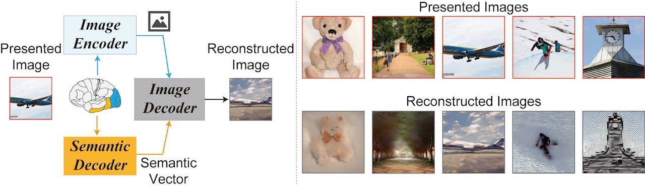
Fig. 9 Stable Diffusion brain signal reconstruction. (Source: Takagi & Nishimito, 2023)#
ImageBind - Holistic AI learning across six modalities#

Fig. 10 ImageBind modalities. (Source: ai.meta.com)#
Definition#
Machine learning at the intersection of engineering, physics, chemistry, computational biology, etc., and core machine learning to improve existing scientific workflows, derive new scientific insight, or bridge the gap between scientific data and our current state of knowledge.
Important here to recall is the difference in approaches between engineering & physics, and machine learning on the other side:
Engineering & Physics#
Models are derived from conservation laws, observations, and established physical principles.
Machine Learning#
Models are derived from data with imprinted priors on the model space either through the data itself or through the design of the machine learning algorithm.
Supervised vs Unsupervised#
There exist 3 main types of modern-day machine learning:
Supervised Learning
Unsupervised Learning
Reinforcement Learning
Supervised Learning#
In supervised learning we have a mapping \(f: X \rightarrow Y\), where the inputs \(x \in X\) are also called features, covariates, or predictors. The outputs \(y \in Y\) are often called the labels, targets, or responses. The correct mapping is then learned from a labeled training set.
with \(N\) the number of observations. Depending on the type of the response vector \(y\), we can then perform either regression, or classification
Some also call it “glorified curve-fitting”
Regression#
In regression, the target \(y\) is real-valued, i.e. \(y \in \mathbb{R}\)
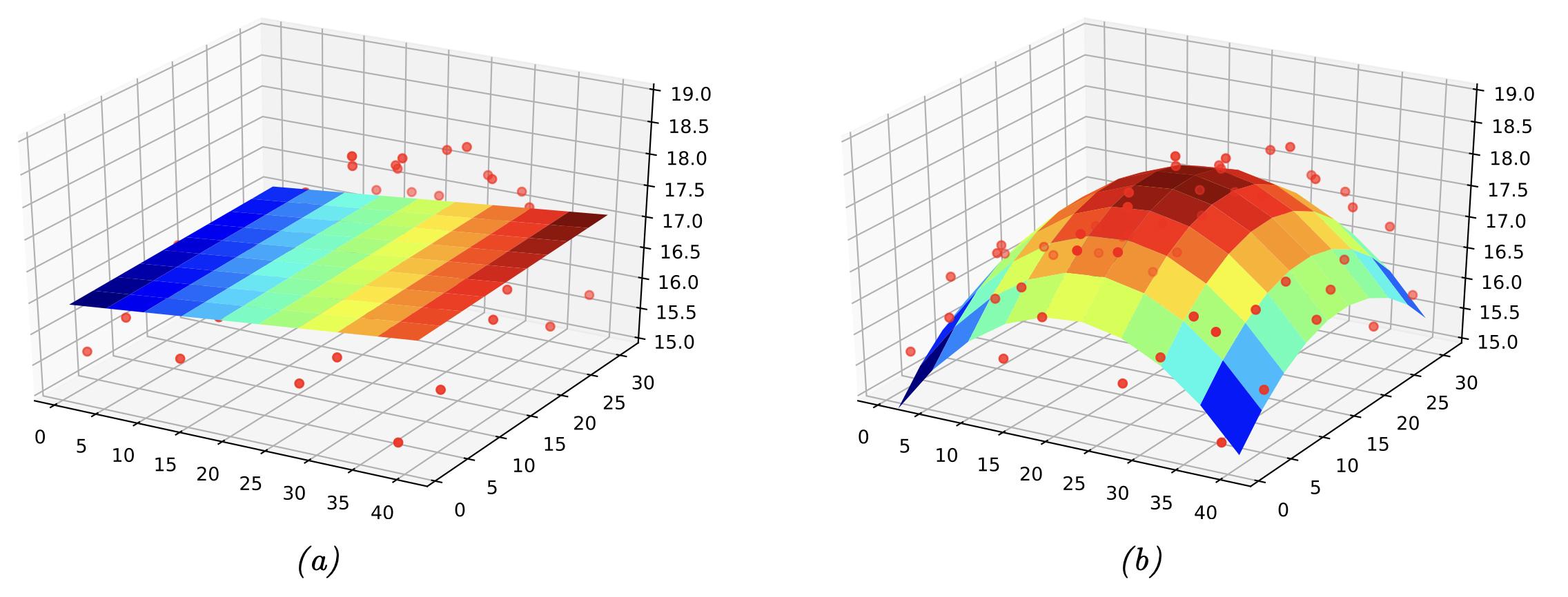
Fig. 11 2D regression example. (Source: [Murphy, 2022], Introduction)#
Example of a response surface being fitted to several data points in 3 dimensions, where the x- and y-axes are a two-dimensional space, and the z-axis is the temperature in the two-dimensional space.
Classification#
In classification, the labels \(y\) are categorical, i.e., \(y \in \mathcal{C}\), where \(\mathcal{C}\) defines a set of classes.
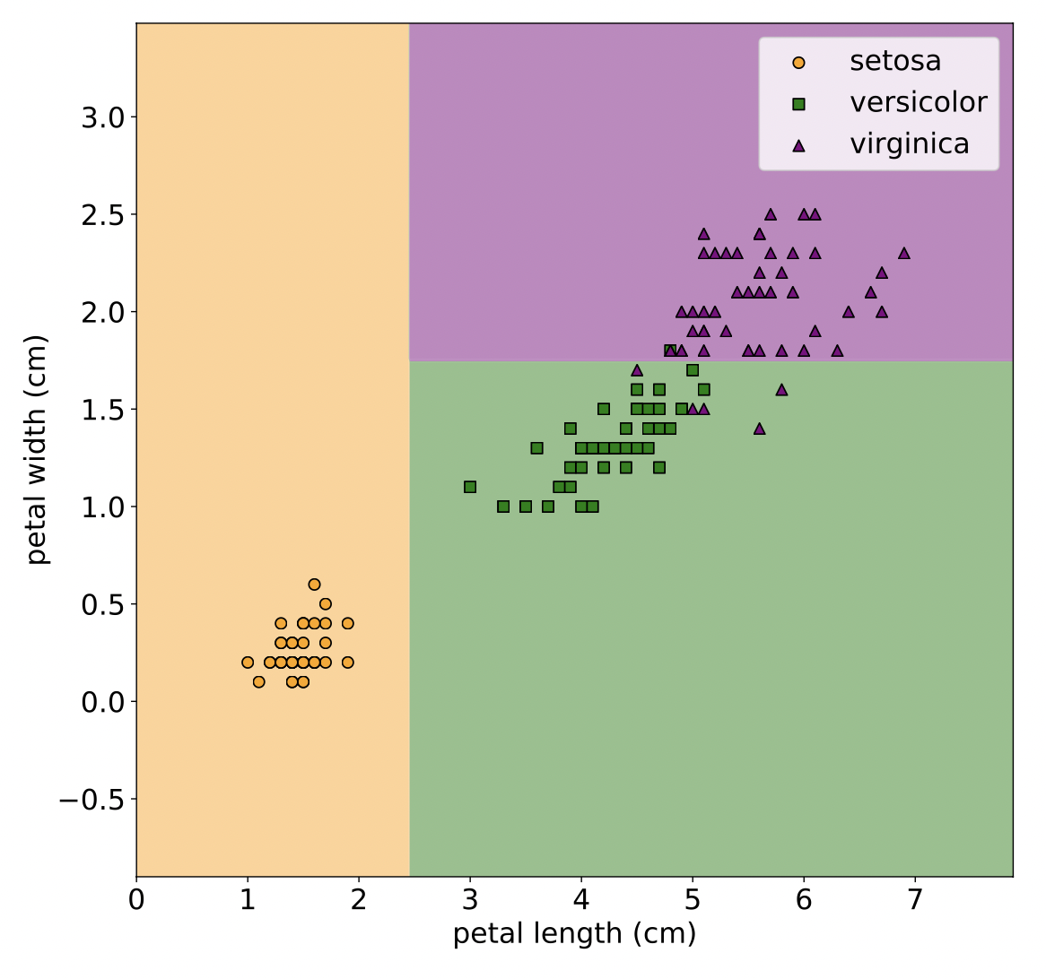
Fig. 12 Classification example. (Source: [Murphy, 2022], Introduction)#
An example of flower classification is where we aim to find the decision boundaries to sort each node into the respective class.
Unsupervised Learning#
In unsupervised learning, we only receive a dataset of inputs.
without the respective outputs \(y_{n}\), i.e. we only have unlabelled data.
The implicit goal here is to describe the system and identify features in the high-dimensional inputs.
Two famous examples of unsupervised learning are clustering (e.g., k-means) and especially dimensionality reduction (e.g., principal component analysis), which is commonly used in engineering and scientific applications.
Clustering of Principal Components#
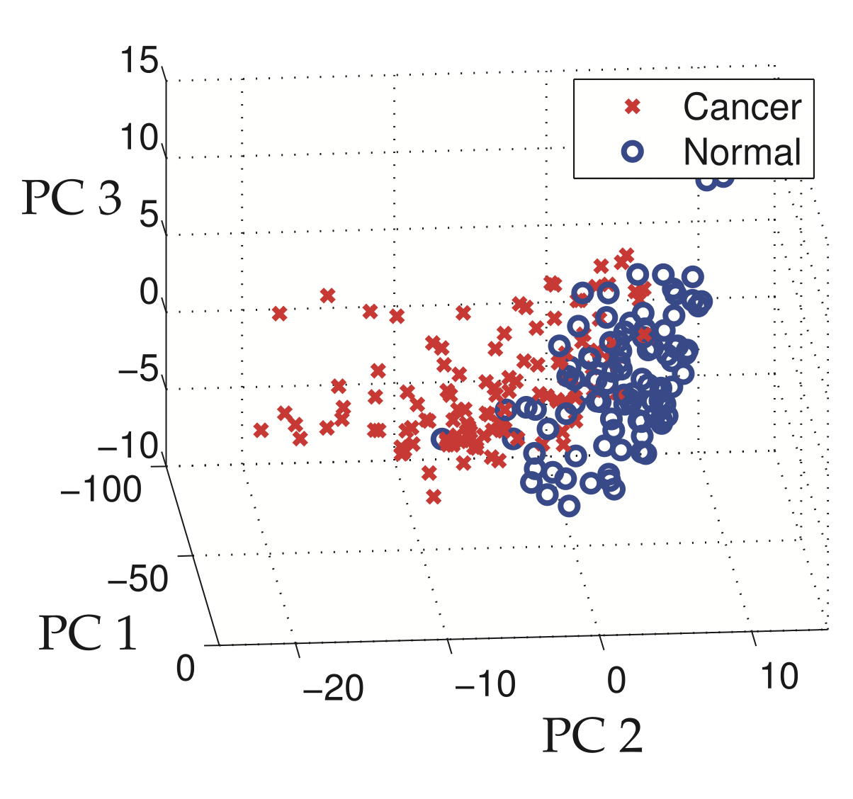
Fig. 13 Clustering based on the principal components. (Source: [Brunton and Kutz, 2019], Section 1.5)#
Combining clustering with principal component analysis to show the samples that have cancer in the first three principal component coordinates.
Supervised vs Unsupervised, the tl;dr in Probabilistic Terms#
Furthermore, the difference can be expressed in probabilistic terms, i.e., in supervised learning, we fit a model over the outputs conditioned on the inputs \(p(y|x)\). In contrast, in unsupervised learning, we fit an unconditional model \(p(x)\).
Reinforcement Learning#
In reinforcement learning, an agent sequentially interacts with an unknown environment to obtain an interaction trajectory \(T\), or a batch thereof. Reinforcement learning then seeks to optimize how the agent interacts with the environment through its actions \(a_{t}\) to maximize a (cumulative) reward function to obtain an optimal strategy.
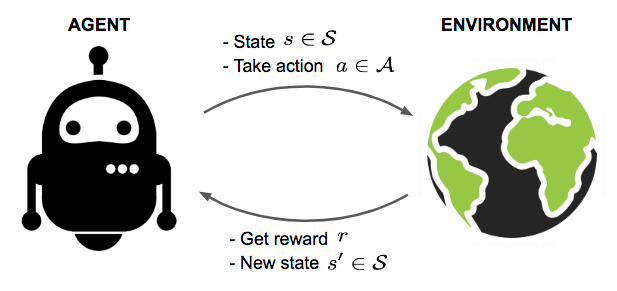
Fig. 14 Reinforcement learning overview. (Source: lilianweng)#
Polynomial Curve Fitting#
Let’s presume we have a simple regression problem, e.g.
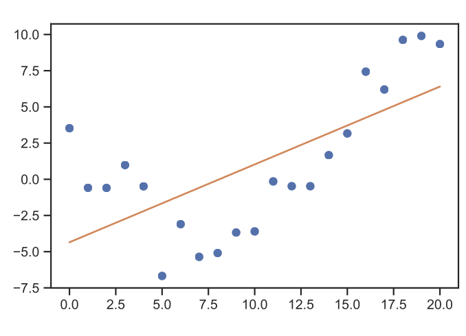
Fig. 15 Linear regression example. (Source: [Murphy, 2022], Introduction)#
Then we have a number of scalar observations \({\bf{x}} = (x_{1}, \ldots, x_{N})\) and targets \({\bf{y}} = (y_{1}, \ldots, y_{N})\). The tool we have probably seen before in the mechanical engineering curriculum is the simple approach to fit a polynomial function
Then a crucial choice is the degree of the polynomial function.
This class of models is called Linear Models because we seek to learn only the linear scaling coefficients \(w_i\), given any choice of basis for the variable \(x\) like the polynomial basis shown here.
We can then construct an error function with the sum of squares approach in which we compute the distance of every target data point to our polynomial.
We then optimize for the value of \(w\).
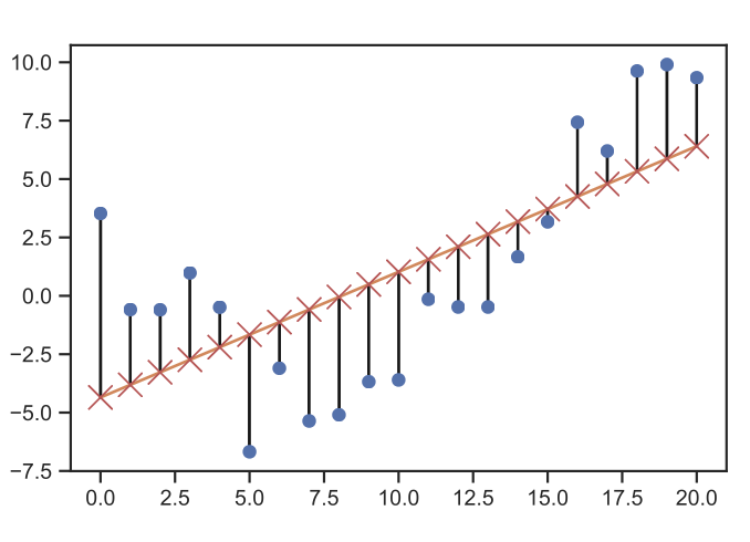
Fig. 16 Linear regression error computation. (Source: [Murphy, 2022], Introduction)#
To minimize this, we then have to take the derivative with respect to the coefficients \(\omega_{i}\), i.e.
which we are optimizing for and by setting to 0, we can then find the minimum
This can be solved by the trusty old Gaussian elimination. A general problem with this approach is that the degree of the polynomial is a decisive factor that often leads to over-fitting and hence makes this a less desirable approach. Gaussian elimination, or a matrix inversion approach, when implemented on a computer, can also be a highly expensive computational operation for large systems.
This is a special case of the Maximum Likelihood method.
Bayesian Curve Fitting#
Recap: Bayes Theorem#
If we now seek to reformulate the curve-fitting in probabilistic terms, we must begin by expressing our uncertainty over the target \(y\) with a probability distribution. For this, we presume a Gaussian distribution over each target where the mean is the point value we previously considered, i.e.
where \(\beta\) corresponds to the inverse variance of the normal distribution \(\mathcal{N}\). We can then apply the maximum likelihood principle to find the optimal parameters \(\mathbf{w}\) with our new likelihood function
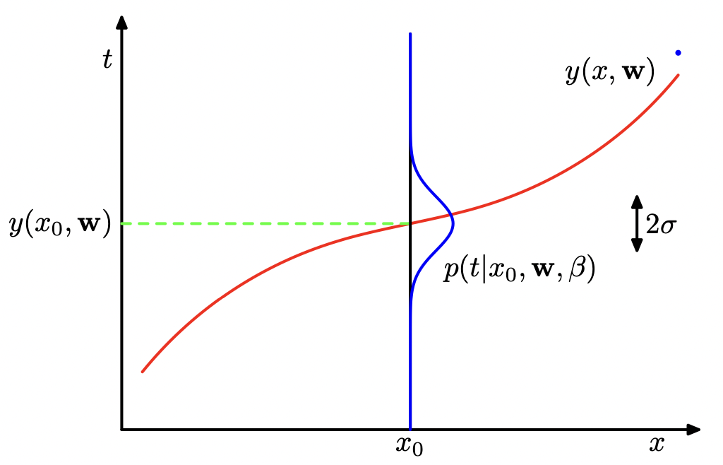
Fig. 17 Bayesian regression example. (Source: [Bishop, 2006], Section 1.2)#
Taking the log-likelihood, we are then able to find the definitions of the optimal parameters
We can then optimize for the \(\mathbf{w}\).
If we consider the special case of \(\frac{\beta}{2}=\frac{1}{2}\), and instead of maximizing, minimizing the negative log-likelihood, then this is equivalent to the sum-of-squares error function.
The herein obtained optimal maximum likelihood parameters \(\mathbf{w}_{ML}\) and \(\beta_{ML}\) can then be resubstituted to obtain the predictive distribution for the targets \(y\).
To arrive at the full Bayesian curve-fitting approach, we must apply the sum and product rules of probability.
Recap: Sum Rules of (disjoint) Probability#
Recap: Product Rules of Probability - for independent events \(A,B\)#
The Bayesian curve fitting formula is hence
with the dependence on \(\beta\) omitted for legibility reasons. This integral can be solved analytically hence giving the following predictive distribution
with mean and variance
and \({\bf{S}}\) defined as
and \({\bf{I}}\) the unit matrix, while \(\phi(x)\) is defined by \(\phi_{i}(x) = x^{i}\). Examining the variance \(s^{2}(x)\), then the benefits of the Bayesian approach become readily apparent:
\(\beta^{-1}\) represents the prediction uncertainty
The second term of the variance is caused by the uncertainty in the parameters \(w\).
Maximum Likelihood & Log-Likelihood#
Formalizing the principle of maximum likelihood estimation, we seek to act similarly to function extrema calculation in high school in that we seek to differentiate our likelihood function, and then find its maximum value by setting the derivative equal to zero.
where \(\mathcal{L}\) is the likelihood function. In the derivation of the Bayesian Curve Fitting approach we have already utilized this principle by exploiting the independence between data points and then taking the log of the likelihood to subsequently utilize the often nicer properties of the log-likelihood
Recap#
Supervised Learning: Mapping from inputs \(x\) to outputs \(y\)
Unsupervised Learning: Only receives the datapoints \(x\) with no access to the true labels \(y\)
Maximum Likelihood Principle
Polynomial Curve Fitting a special case
Wasteful of training data, and tends to overfit
Bayesian approach less prone to overfitting
Further References#
Using AI to Accelerate Scientific Discovery - inspirational video by Demis Hassabis