5. Tricks of Optimization#
Learning outcome
What is under- and overfitting explained through the bias-variance tradeoff?
Why do we need data splitting, and how do we typically approach it?
Name three classes of approaches for improving the speed and/or generalization of learning algorithms.
What is the “recipe” for ML?
This lecture introduces fundamental concepts in data science, such as the bias-variance tradeoff, and complements them with a collection of practical tools for designing and optimizing machine learning models.
5.1. Recap#
5.1.1. Linear Regression (revised)#
Looking back to Lecture 1, the simplest linear model for input \(x \in \mathbb{R}\) and target \(y \in \mathbb{R}\) is
We remind the reader that the polynomial linear regression
also represents a linear model in terms of its parameters \(\vartheta_i\) (not to be confused with the first order model for \(x \in \mathbb{R}^n\)). The general linear regression could be any linear combination of x-values lifted to a predefined basis space, e.g., exponent, sine, cosine, etc.:
5.1.2. Nonlinear Regression#
Any function that is more complicated than linear regarding its parameters \(\vartheta\), e.g.
5.2. Under- and Overfitting#
Dealing with real-world data containing measurement noise, we often run either into under- or overfitting, depending on the expressivity of the model. Looking at the figure below, the left regression example corresponds to \(h(x) = \vartheta_0 + \vartheta_1 \cdot x\), and the left classification example corresponds to logistic regression.
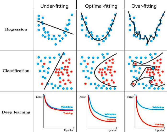
Fig. 5.1 Under- and overfitting (Source: Techniques for handling underfitting and overfitting in Machine Learning)#
5.2.1. Bias-Variance Tradeoff#
Typically, under- and overfitting are analyzed through the lens of the bias-variance decomposition. We define the average model \(h_{ave}(x)\) as the model obtained by drawing an infinite number of datasets of size \(m\), training on them, and then averaging their predictions at a given \(x\).
Bais Error: Difference between \(h_{ave}(x^{(i)})\) and the correct target value \(y^{(i)}\).
Variance Error: Variability of the model predictions at a given \(x\).
Irreducible Error: Originates from the noise in the measurements. Given a corrupted dataset, this error cannot be reduced with ML.
In the figure below, each point corresponds to the prediction of a model trained on a different dataset.
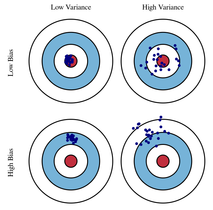
Fig. 5.2 Bias vs. variance tradeoff (Source: Understanding the Bias-Variance Tradeoff)#
Mathematically, the bias-variance decomposition relies on a decomposition of the expected loss over the dataset \(S=\left\{(x^{(i)}, y^{(i)})\right\}_{i=1,...m}\). The assumption is that there is a true underlying relationship between \(x\) and \(y\) given by \(y=\tilde{h}(x)+\epsilon\) where the noise \(\epsilon\) is normally distributed, i.e., \(\epsilon \sim \mathcal{N}(0,\sigma_{\epsilon})\). We try to approximate \(\tilde{h}\) by our model \(h_{\vartheta}\) which results in the error
Using \(y=\tilde{h}(x)+\epsilon\) and the average model \(h_{ave}(x)=\mathbb{E}_S[h_{\vartheta}(x)]\), the error can be decomposed into its bias and variance components as
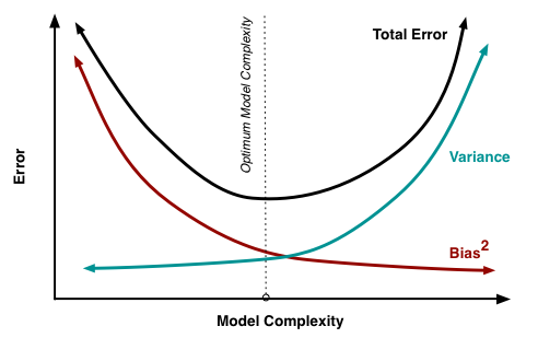
Fig. 5.3 Error vs model complexity (Source: Understanding the Bias-Variance Tradeoff)#
Given the true model and enough data to calibrate it, we should be able to reduce both the bias and variance terms to zero. However, working with imperfect models and limited data, we strive for an optimum in terms of model choice.
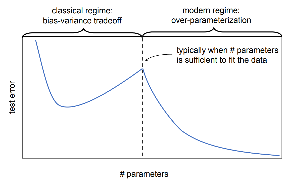
5.2.2. Advanced Topics: Double Descent#
In recent years, machine learning models have grown extremely large, e.g., GPT-4 with an estimated 1.5T parameters. Empirical observations demonstrate that contrary to the theory behind the bias-variance tradeoff, if the number of parameters is too overparametrized, model performance starts improving again. Indeed, for many practical applications, this regime has not been fully explored, and making ML models larger seems to improve performance further, consistently with The Bitter Lesson by R. Sutton.
In contrast to linear models, almost all such functions result in a non-convex loss surface w.r.t. the parameters \(\vartheta\).
5.3. Data Splitting#
To train a machine learning model, we typically split the given data \(\left\{x^{(i)}, y^{\text {(i)}}\right\}_{i=1,...m}\) into three subsets.
Training: Used for optimizing the parameters of a model.
Validation: Used for evaluating performance during hyperparameter tuning and/or model selection.
Testing: Used for evaluating the performance at the very end of tuning the model and its parameters.
Given that the dataset is large enough, typical splits of the training/validation/testing data range from 80/10/10 to 60/20/20. If data is very limited, we might not want to sacrifice separate data for validation. Then, we could use Cross Validation.
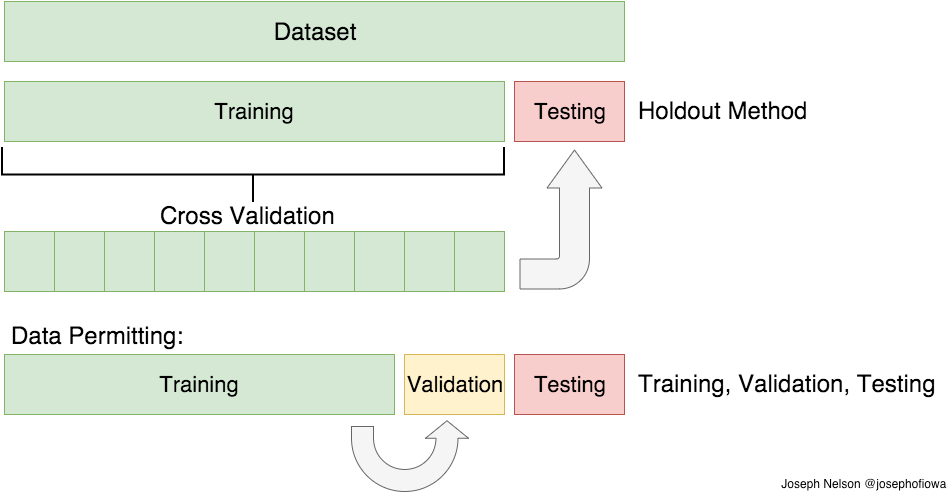
Fig. 5.5 Data splitting (Source: Train/Test Split and Cross Validation in Python)#
5.3.1. \(k\)-fold Cross Validation#
\(k\)-fold cross validation is a method for model selection which does not require a separate validation data split. Model selection can mean choosing the highest polynomial degree in polynomial linear regression, or deciding on the learning algorithms altogether, e.g. linear regression vs using a neural network. Cross validation is particularly relevant if we have a very small dataset, say 20 measurements, and we cannot afford a validation split. Note that without validation data, we cannot do any model selection or hyperparameter tuning.
If we split a dataset into \(k\) disjoint subsets, we could train a model \(k\) times each time, excluding a different subset. We could then evaluate the model performance on the respective left-out subset for each of the \(k\) trained models, and by averaging the results, we get a good estimate of the model performance given the particular model choice. If we apply this procedure to \(N\) different models, we can choose the most suitable model based on its average performance. Once we have chosen the model, we can then train it further on the whole training set.
If we can afford a validation split, we would train each of the \(N\) models only once instead of \(k\) times, and we would pick the best one by evaluating the performance on the validation split.
5.4. Regularization#
One possibility to counteract overfitting while still having an expressive model is regularization. There are many approaches belonging to the class of regularization techniques.
Adding a regularization term to the loss - an additional term penalizing large weight values:
L1 regularization - promotes sparsity:
(5.7)#\[J_{L1}(\vartheta) = J(\vartheta) + \alpha_{L1} \cdot \sum_{i=1}^{\#params} |\vartheta_i|\](squared) L2 regularization - takes information from all features:
(5.8)#\[J_{L2}(\vartheta) = J(\vartheta) + \alpha_{L2} \cdot \sum_{i=1}^{\#params} \vartheta_i^2\]Dropout: randomly set some parameters to zero, e.g., 20% of all \(\vartheta_i\). This way, the model learns to be more redundant and, at the same time, improves generalization. Dropout reduces co-adaptation between terms of the model. Also, this technique is very easy to apply.
Eary stopping: Stop training as soon as the validation loss starts increasing, i.e., overfitting begins. This is also a very common and easy technique.
etc.
\(l_p\) norm
To better understand the additional regularization loss terms, we look at the general \(l_p\) norm of the weight vector \(w\in \mathbb{R}^m\) (\(w\equiv \vartheta\)):
In the special case \(p=1\), we recover the L1 regularization term, and the squared version of \(p=2\) corresponds to the L2 regularization term. Other special case is \(p \to \infty\) leading to \(||w||_{\infty}= \max \left\{ |w_1|,|w_2|,...,|w_{n}| \right\}\). We see that with increasing \(p\), the larger terms dominate.
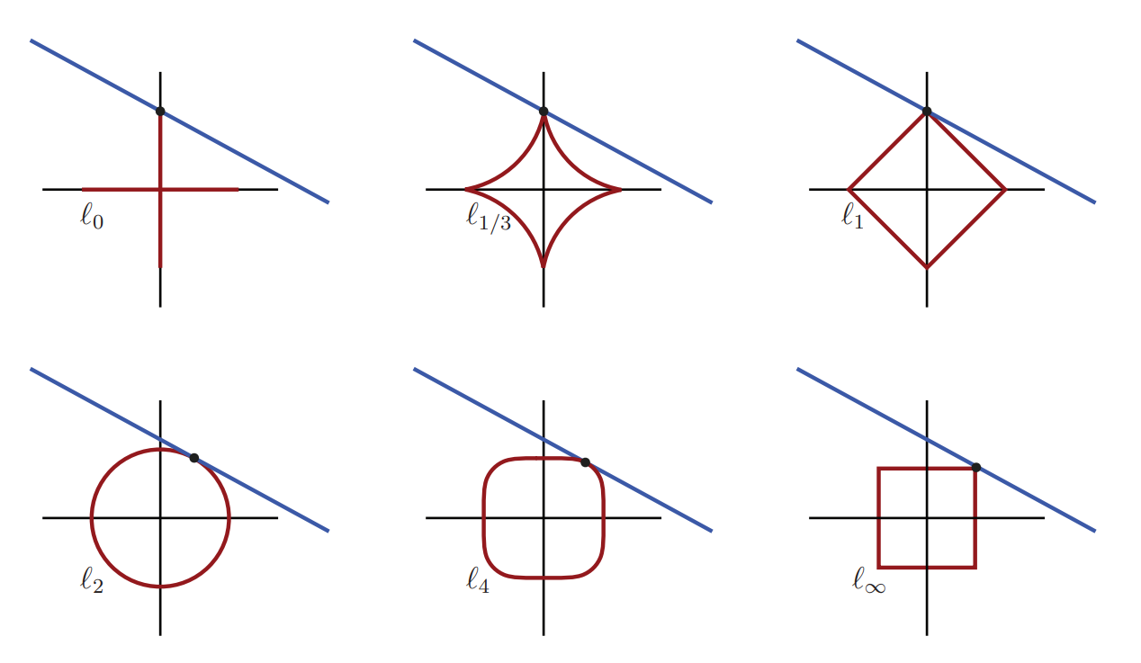
Fig. 5.6 The blue line represents the solution set of an under-determined system of equations. The red curve represents the minimum-norm level sets that intersect the blue line for each norm. For norms \(p=0,...,1\), the minimum-norm solution corresponds to the sparsest solution, with only one active coordinate. For \(p \ge 2\), the minimum-norm solution is not sparse, and both coordinates are active. (Source: [Brunton and Kutz, 2019], Fig. 3.9)#
5.5. Input/Output Normalization and Parameter Initialization#
The idea behind input/output normalization and parameter initialization is simply to speed up the learning process, i.e., reduce the number of gradient descent iterations by bringing all values to the same order of magnitude. Normalization and initialization will be further discussed in the Deep Learning lectures towards the end of this course.
5.5.1. Case Study 1 - Input Normalization#
We choose a linear model
between the input \(x\in \mathbb{R}\) and output \(y\in \mathbb{R}\). In the case of the MSE loss, the gradient w.r.t. the parameters becomes
Assume that this linear model coincides with the true underlying model having \(\vartheta^{true} = [\vartheta^{true}_0, \vartheta^{true}_1] = [1, 1]\). We are also given that the input \(x\) has a mean and standard deviation over the dataset equal to \(0\) and \(0.001\).
If we start a GD optimization from an initial \(\vartheta^0 = [0, 0]\), we immediately see that the average gradient w.r.t \(\vartheta_1\) will be 1000 times smaller than the one for \(\vartheta_0\) because of the multiplication with \(x\). Thus, we would need a learning rate small enough for \(\vartheta_0\) and, at the same time, enough iterations for the convergence of \(\vartheta_1\).
To alleviate this problem, we can normalize the inputs to zero mean and variance of one. This can be achieved by precomputing the mean \(\mu=1/m \sum_{i=1}^m x^{(i)}\) and variance \(\sigma^2=1/m \sum_{i=1}^m \left(x^{(i)}-\mu \right)^2\) of the inputs, and then transforming each input to
If \(x \in \mathbb{R}^n\) with \(n > 1\), we would do that to each dimension individually.
In signal processing, a similar transformation is called the whitening transformation - the difference is that whitening considers correlations between the dimensions.
Note: Normalization should also be applied to the outputs \(y\) as a similar problem of unfavorable magnitudes can also be observed for them.
5.5.2. Case Study 2 - Parameter Initialization#
Given is the already normalized input \(x\in \mathbb{R}^n\) with \(n>>1\) and the true underlying linear model of the form
with \(\vartheta^{true} = [0.1, ..., 0.1]\). If we start a GD optimization from an initial \(\vartheta^0 = [0,1,2, ..., n]\), we would run into a problem. To make training work, we would again need a small learning rate to move from the initial \(\vartheta^0_0=0\) to \(\vartheta^{true}_0=0.1\), which would then require \(\mathcal{O}(n)\) more updates to move \(\vartheta^0_n=n\) to \(\vartheta^{true}_n=0.1\).
Xavier initialization has been proposed to alleviate this type of issue. It essentially initializes the parameters by drawing them from \(\mathcal{N}(0,1/n)\), i.e., a zero-centered normal distribution with variance \(1/n\). This way we:
Choose the terms of \(\vartheta^0\) in the same order of magnitude, resulting in a similar weighting of each term in the model (given that the inputs \(x\) are normalized beforehand).
End up with outputs \(h(x)\) distributed close to a standard normal distribution. And if we normalize the target \(y\) beforehand, it would be in the same order of magnitude as \(h(x)\).
5.6. Hyperparameter Search#
A hyperparameter is a parameter that controls other parameters. Typically, we cannot afford to optimize hyperparameters with gradient-based methods and resort to derivative-free optimization methods - see the lecture on Optimization.
One of the most important hyperparameters in 1st order gradient-based optimization is the learning rate \(\eta\). We typically tune the learning rate by looking at the so-called training curves. To see the impact of different values of the learning rate on the validation loss, look at the following figure.
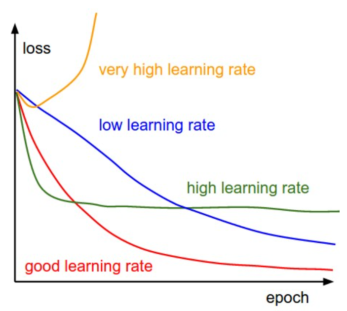
Fig. 5.7 Effect of learning rate on training curves (Source: CS231n CNNs for Visual Recognition)#
Further hyperparameters are, e.g., the choice of model, the optimizer itself, and batch size in SGD. You will see many of them related to each model later in the lecture.
5.6.1. Learning Rate Scheduling#
We want to be able to dynamically adjust the learning rate \(\eta\) towards a time-dependent learning rate \(\eta(t)\). Some common schedulers for progressively decreasing the learning rate include
Going through the different proposed options in order:
Piecewise constant: Decrease whenever optimization progress begins to stall.
Exponential decay: More aggressive; can lead to premature stopping.
Polynomial decay: Well-behaved when \(\alpha = 0.5\).
Using a time-dependent learning rate, the optimization is more stable than the corresponding SGD alternative Fig. 4.7.
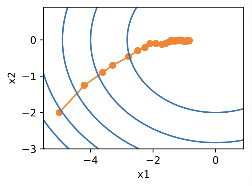
Fig. 5.8 Training with learning rate scheduling (Source: [Zhang et al., 2021], here)#
5.6.2. Recipe for Machine Learning#
If you are wondering how all of that fits together, Andrew Ng suggests the following general workflow (dev=validation split).
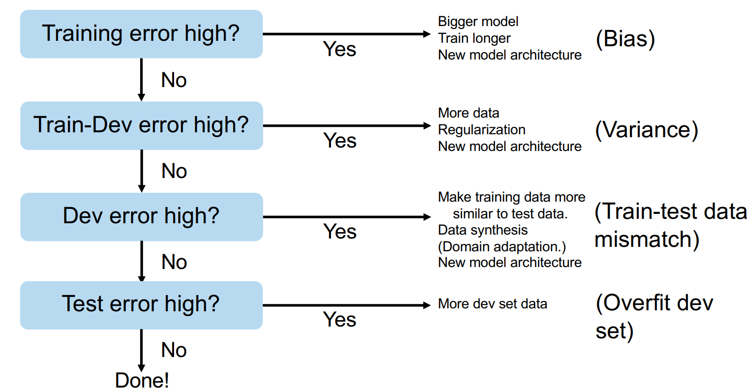
Fig. 5.9 Recipe for ML (Source: Nuts and Bolts of Building Applications using Deep Learning)#
And a piece of practical advice from Matthias Niessner (computer vision professor at TUM):
Train the model on a single data point to essentially learn it by heart. This way, you validate that the model and training pipeline work correctly.
Train the model on a few samples. Validates that multiple inputs are handled correctly.
Move from the overfitting regime to full training.
5.7. Further References#
Under- and Overfitting
[Ng, 2022], Chapter 8
[Goodfellow et al., 2016], Chapter 5
Understanding the Bias-Variance Tradeoff, S. Fortmann-Roe, 2012
Data Splitting and Regularization
[Ng, 2022], Chapter 9
[Murphy, 2022], Sections 4.5 and 13.5
[Goodfellow et al., 2016], Chapters 5 and 7
Normalization and Initialization
[Murphy, 2022], Section 13.4
[Goodfellow et al., 2016], Section 8.4
Hyperparameters
[Murphy, 2022], Section 13.4
[Goodfellow et al., 2016], Section 11.4