10. Convolutional Neural Networks#
Learning outcome
Which parameters define a convolutional kernel?
Which pooling layers did you learn?
10.1. Limitations of MLP#
In the lecture Multilayer Perceptron, we saw how the Multilayer Perceptron (a.k.a. Feed-Forward Neural Network or Fully Connected Neural Network) generalizes linear models by stacking many affine transformations and placing nonlinear activation functions in between. Also, by the Universal Approximation Theorem, we saw that such a construction is enough to learn any function. But is an MLP always practical?
In this subsection, we will concentrate on working with images. Imagine that we have an image with 1000x1000 pixels and 3 RGB channels. If we take an MLP with one hidden layer of size 1000, this means that the weight matrix applied to the input would have 3 billion parameters to map all 3M inputs to each of the 1k neurons in layer 1. This number is significantly large for most modern consumer hardware, and thus, such a network could not be easily trained or deployed.
MLPs are, in a sense, the most brute-force deep learning technique. By directly connecting all input entries to all next-layer neurons, we don’t introduce any model bias, but this is not necessarily the best approach for image data.
The core idea of Convolutional Neural Networks (CNNs) is to introduce weight sharing, i.e., different regions of the image are treated with the same weights.
10.2. Convolution#
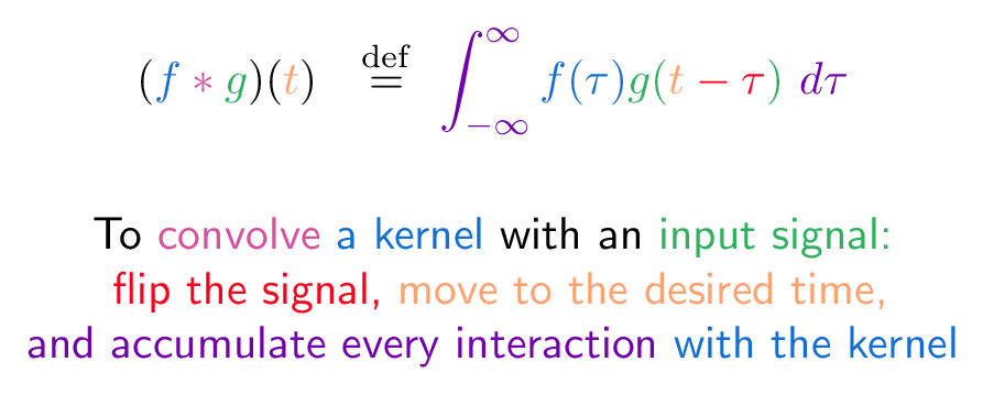
Fig. 10.1 Continuous convolution equation (Source: Intuitive Guide to Convolution)#
Applying a convolution filter (a.k.a. kernel) to a 2D image might look like this.
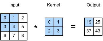
Fig. 10.2 Image convolution (Source: [Zhang et al., 2021], here)#
10.2.1. Filters#
In image processing, specific (convolution) kernels have a well-understood meaning. Examples include:
Edge detection
Sharpening
Mean blur
Gaussian blur
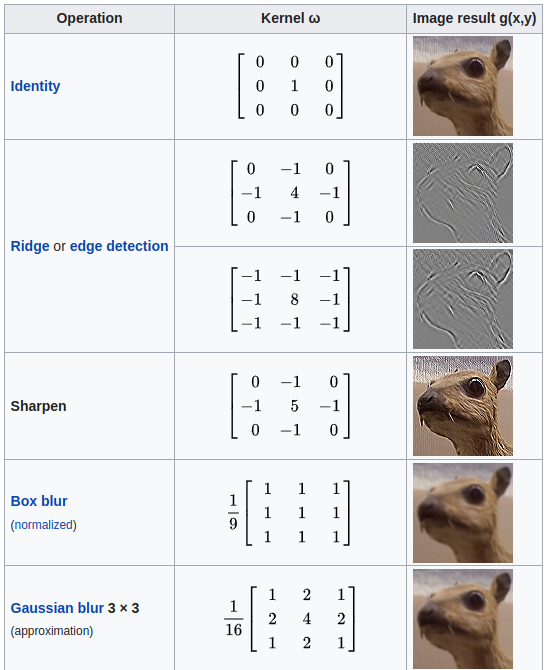
Fig. 10.3 Examples of convolutional kernels (Source: Wikipedia)#
The kernels is modern deep learning “react” to features like these:
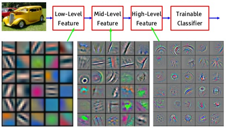
Fig. 10.4 Reconstructed patterns that cause high activations in a given feature map (Image credit: Yann LeCun 2016, adapted from Zeiler & Fergus 2013)#
10.3. Dimensions of a Convolution#
If you got excited about CNNs and open the PyTorch documentation of the corresponding torch.nn.Conv2d section, you will find the following notation:
Input shape: \((N, C_{in}, H_{in}, W_{in})\)
Output shape: \((N, C_{out}, H_{out}, W_{out})\)
Here, \(N\) is the batch size, \(C\) the number of channels, e.g. 3 for an RGB input image, \(H\) is the height, and \(W\) the width of an image. Using this notation we can compute the output height \(H_{out}\) and output width \(W_{out}\) of a CNN layer:
Here, \(\lfloor \cdot \rfloor\) denotes the floor operator. Let’s look at what each of these new terms means.
10.3.1. Padding#
Applying a convolution directly to an image would result in an image of a smaller height and width. To counteract that, we pad the image height and width, for example, with zeros. With the proper padding (referred to as same convolution), one can stack hundreds of convolution layers without changing the width and height. The padding can be different along the width and height dimensions; we denote width and height padding with \(\text{padding}[0]\) and \(\text{padding}[1]\), respectively. The original convolution corresponds to \(\text{padding}=0\).
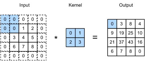
Fig. 10.5 Convolution with zero padding of size one on each side (Source: [Zhang et al., 2021], here)#
Another reason for padding is to use the corner pixels equally often as other pixels. The image below shows how often a pixel would be used by a convolution kernel of size 1x1, 2x2, and 3x3 without padding.
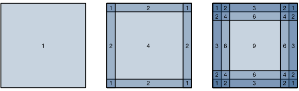
Fig. 10.6 Convolution without padding (Source: [Zhang et al., 2021], here)#
Two commonly used terms regarding padding are the following:
valid convolution: no padding
same convolution: \(H_{in}=H_{out}, \; W_{in}=W_{out}\).
10.3.2. Stride#
If we want to reduce the overlap between kernels and also reduce \(W\) and \(H\) of the outputs, we can introduce a \(\text{stride}>1\) variable. \(\text{stride}=1\) results in the original convolution. In the image below we see \(\text{stride}=\text{Array}([2, 3])\).
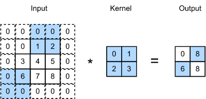
Fig. 10.7 Convolution with stride (Source: [Zhang et al., 2021], here)#
10.3.3. Dilation#
This is a less common operation that works well for detecting large-scale features. \(\text{dilation}=1\) corresponds to the original convolution.
Fig. 10.8 Convolution with dilation of size 2 (Source: vdumoulin/conv_arithmetic)#
10.4. Pooling#
You can think of a convolution filter as a feature extraction transformation similar to the basis expansion with general linear models. Here, the basis itself is learned via CNN layers.
If we are interested in image classification, we don’t just want to transform the input features but also extract / select the relevant information. This is done by pooling layers in between convolution layers. Pooling layers don’t have learnable parameters, and they inevitably reduce dimensionality. Typical examples are:
max / min pooling
mean pooling (averaging)
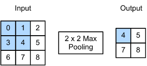
Fig. 10.9 Max pooling (Source: [Zhang et al., 2021], here)#
10.4.1. Channels#
Each convolutional kernel operates on all \(C_{in}\) input channels, resulting in a number of parameters per kernel being \(C_{in} \cdot \text{kernel_size}[0] \cdot \text{kernel_size}[1]\). Having \(C_{out}\) number of kernels results in a number of parameters per convolutional layer given by
The following is an example with two input channels, one output channel, and a 2x2 kernel size.
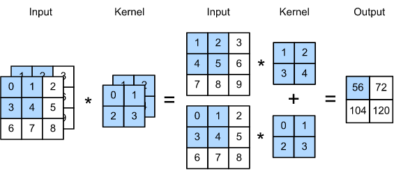
Fig. 10.10 Convolution of a 2-channel input with a 2x2 kernel (Source: [Zhang et al., 2021], here)#
10.5. Modern CNNs#
A typical CNN would look something like the following.
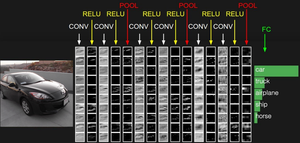
Fig. 10.11 Modern CNN (Source: cs231n, CNN lecture)#
We now head to a historical overview of the trends since the beginning of the deep learning revolution with AlexNet in 2012.
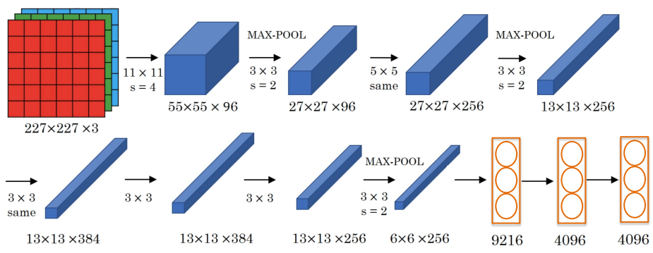
10.5.1. AlexNet (2012)#
Characteristics:
rather large filters of size 11x11
first big successes of ReLU
60M parameters
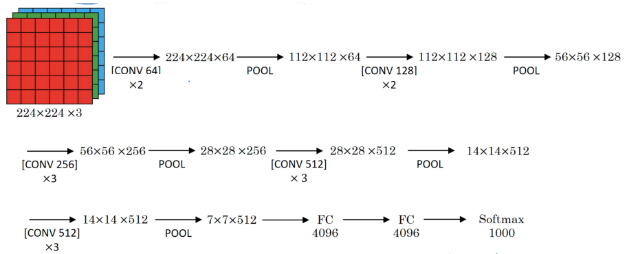
10.5.2. VGGNet (2014)#
Characteristics:
much simpler structure
3x3 convolutions, stride 1, same convolutions
2x2 max pooling
deeper
138M parameters
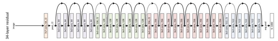
10.5.3. ResNet (2016)#
Characteristics:
allows for very deep networks by introducing skip connections
this mitigates the vanishing and exploding gradients problem
ResNet-152 (with 152 layers) has 60M parameters
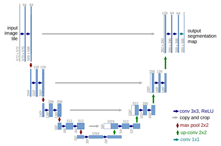
10.5.4. U-Net (2015)#
Characteristics:
for image segmentation
skip connections
10.5.5. Advanced Topics: ConvNext (2022) and ConvNextv2 (2023)#
Characteristics:
since the Vision Transformer, many people believe that the inductive bias of translational invariance encoded in a convolution is too restrictive for image classification. However, the release of the ConvNext model (“A ConvNet for the 2020s”, Liu et al. 2022) points in the direction that many innovations have been made on improving transformers, e.g. the GELU activations, and if we simply apply some of them to CNNs, we also end up with state-of-the-art results.
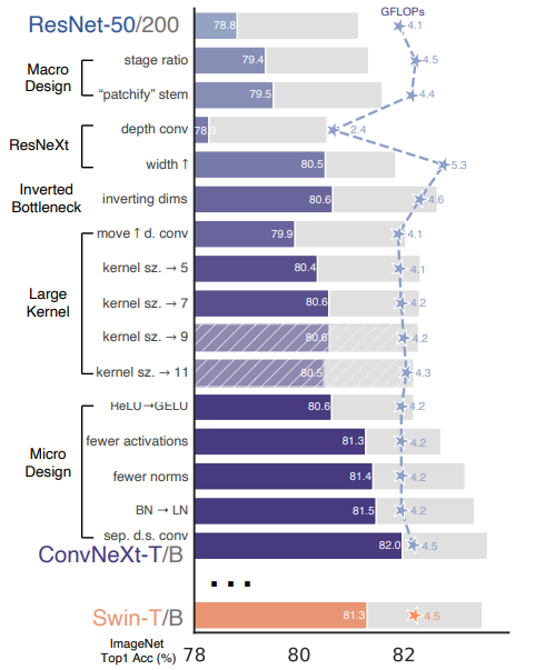
Fig. 10.16 ConvNext ablations (Source: A ConvNet for the 2020s)#
The successor paper of ConvNext -> ConvNextv2 came out one week before this lecture in WS22/23 :)
10.6. Further References#
[Goodfellow et al., 2016], Chapter 9
[Zhang et al., 2021], Chapters “Convolutional Neural Networks” and “Modern Convolutional Neural Networks”