2. Gaussian Mixture Models#
Learning outcome
Explain the product/sum rule of probabilities and Bayes rule.
Explain the assumption behind GMMs and point to the respective terms in the GMM equation.
Give an intuition on why GMMs do not have a closed-form solution and sketch the steps of the most commonly used optimization method for GMMs.
This lecture first recaps Probability Theory and then introduces Gaussian Mixture Models (GMM) for density estimation and clustering.
Concerning the following lecture introducing sampling, GMMs and sampling methods (e.g. MCMC) are two complementary approaches:
GMMs estimate the probability density of a given set of samples
MCMC generates samples from a given probability density
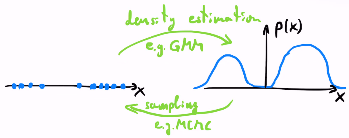
Fig. 2.1 Density estimation vs sampling.#
But first, we revise Probability Theory.
Note: To refresh your math knowledge, we have prepared a set of exercises incl. solutions under Preliminary Knowledge.
2.1. Probability Theory#
2.1.1. Basic Building Blocks#
\(\Omega\) - sample space; the set of all outcomes of a random experiment.
\(\mathbb{P}(E)\) - probability measure of an event \(E \in \Omega\); a function \(\mathbb{P}: \Omega \rightarrow \mathbb{R}\) satisfies the following three properties:
\(0 \le \mathbb{P}(E) \le 1 \quad \forall E \in \Omega\)
\(\mathbb{P}(\Omega)=1\)
\(\mathbb{P}(\cup_{i=1}^n E_i) = \sum_{i=1}^n \mathbb{P}(E_i) \;\) for disjoint events \({E_1, ..., E_n}\)
\(\mathbb{P}(A, B)\) - joint probability; probability that both \(A\) and \(B\) occur simultaneously.
\(\mathbb{P}(A | B)\) - conditional probability; probability that \(A\) occurs, if \(B\) has occurred.
Product rule of probabilities:
Sum rule of probabilities:
(2.3)#\[\mathbb{P}(A)=\sum_{B}\mathbb{P}(A, B)\]Bayes rule: solving the general case of the product rule for \(\mathbb{P}(A)\) results in:
(2.4)#\[ \mathbb{P}(B|A) = \frac{\mathbb{P}(A|B) \mathbb{P}(B)}{\mathbb{P}(A)} = \frac{\mathbb{P}(A|B) \mathbb{P}(B)}{\sum_{i=1}^n \mathbb{P}(A|B_i)\mathbb{P}(B_i)}\]\(p(B|A)\) - posterior
\(p(A|B)\) - likelihood
\(p(B)\) - prior
\(p(A)\) - evidence
2.1.2. Random Variables and Their Properties#
Random variable (r.v.) \(X\) is a function \(X:\Omega \rightarrow \mathbb{R}\). This is the formal way to move from abstract events to real-valued numbers. \(X\) is essentially a variable that does not have a fixed value but can have different values with certain probabilities.
Continuous r.v.s:
\(F_X(x)\) - Cumulative distribution function (CDF); probability that the r.v. \(X\) is smaller than some value \(x\):
(2.5)#\[F_X(x) = \mathbb{P}(X\le x), \quad \text{with } F_X(-\infty)=0, \; F_X(\infty)=1\]\(p_X(x)\) - Probability density function (PDF):
(2.6)#\[p_X(x)=\frac{dF_X(x)}{dx}\ge 0 \;\text{ and } \; \int_{-\infty}^{+\infty}p_X(x) dx =1\]
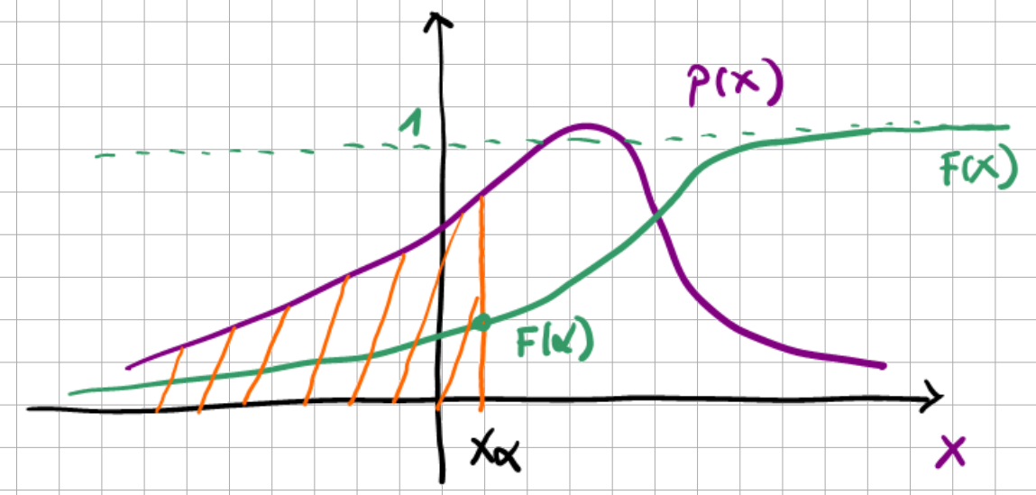
Fig. 2.2 PDF and CDF functions.#
Discrete r.v.s:
Probability mass function (PMF) - same as the pdf but for a discrete r.v. \(X\). Integrals become sums.
\(\mu = E[X]\) - mean value or expected value
(2.7)#\[E[X] = \int_{-\infty}^{+\infty}x \, p_X(x) \, dx\]\(\sigma^2 = Var[X]\) - variance
(2.8)#\[Var[X] = \int_{-\infty}^{+\infty}x^2 \, p_X(x) \, dx = E[(X-\mu)^2]\]\(Cov[X,Y]=E[(X-\mu_X)(Y-\mu_Y)]\) - covariance
Change of variables - if \(X \sim p_X\) and \(Y=h(X)\), then the distribution of \(Y\) becomes:
(2.9)#\[p_Y(y)=p_X(x)\left|\frac{\text{d}x}{\text{d}y}\right| = p_X(h^{-1}(y)) \left|\frac{\text{d}h^{-1}(y)}{\text{d}y}\right|\]
Exercise: Change of Variables
Given the r.v. \(X\) with pdf \(p_X(x)=3x^2\) defined on \(X \in (0,1)\) and the function \(Y=X^2\), find the pdf of \(Y\). Hint: use \(X=h^{-1}(Y)\) as shown here.
2.1.3. Catalogue of Important Distributions#
Discrete
Binomial, \(X\in\{0,1,...,n\}\). Describes how often we get \(k\) positive outcomes out of \(n\) independent experiments. Parameter \(\lambda\) is the success probability of each trial.
(2.10)#\[p(x=k|n, \lambda)=\binom{n}{k}\lambda^k(1-\lambda)^{n-k}, \quad \text{ with } k\in \{0,1,2,..., n\}.\]With the binomial coefficient \(\binom{n}{k}=\frac{n!}{k!(n-k)!}\).
Bernoulli - special case of Binomial with \(n=1\).
Categorical - generalizes Bernoulli to a categorical random variable with \(k\) categories each with probability \(\pi_i\ge 0\) for \(i \in \{1,...,k\}\), such that \(\sum {\pi_i}=1\).
(2.11)#\[\begin{split} \begin{align} p(x=i | \mathbb{\pi}) &=\pi_i\\ &= \prod_{i=1}^k \pi_i^{[x=i]} \end{align} \end{split}\]The two pdf formulations above are equivalent, and the second one uses the Iverson bracket.
Multinomial - a generalization of the Binomial and the Categorical distributions. It models the number of occurrences for each of \(k\) classes when sampling from a categorical distribution is repeated \(n\) times. For \(k=2, n=1\), this becomes Bernoulli; for \(k> 2,n=1\), it is the Categorical; for \(k=2, n>1\), it is the Binomial.
(2.12)#\[p(x_i,...,x_k | n, \mathbf{\pi}) = \frac{n!}{x_1! \dots x_k!} \pi_1^{x_i} \dots \pi_k^{x_k}\]Here, \(x_i\) denotes the number of occurrences of class \(i\), with \(\sum x_i=n\) and \(x_i \ge 0\).
Continuous
Normal (aka Gaussian), \(X \in \mathbb{R}\).
(2.13)#\[p(x| \mu, \sigma)=\mathcal{N}(x|\mu, \sigma^2) = \frac{1}{\sqrt{2 \pi \sigma^2}}\exp\left(-\frac{(x-\mu)^2}{2\sigma^2}\right)\]Multivariate Gaussian \(\mathcal{N}(\mathbf{\mu}, \mathbf{\Sigma})\) of \(\mathbf{X}\in \mathbb{R}^n\) with mean \(\mathbf{\mu}\in \mathbb{R}^n \) and covariance \(\mathbb{\Sigma} \in \mathbb{R}_{+}^{n\times n}\).
(2.14)#\[p_X(x)= \frac{1}{(2\pi)^{n/2}\sqrt{\det (\mathbf{\Sigma})}} \exp \left(-\frac{1}{2}(\mathbf{x}-\mathbf{\mu})^{\top}\mathbf{\Sigma}^{-1}(\mathbf{x}-\mathbf{\mu})\right).\]
2.1.4. Exponential Family#
The exponential family of distributions is a large family of distributions with shared properties, some of which we have already encountered in the previous lecture. Prominent members of the exponential family include:
Bernoulli
Gaussian
Dirichlet
Gamma
Poisson
Beta
At their core, all members of the exponential family fit the same general probability distribution form:
where the individual components are:
\(\eta\) - natural parameter
\(t(x)\) - sufficient statistic
\(h(x)\) - probability support measure
\(a(\eta)\) - log normalizer; guarantees that the probability density integrates to 1.
If you are unfamiliar with the concept of probability measures, then \(h(x)\) can safely be disregarded. Conceptually it describes the area in the probability space over which the probability distribution is defined.
Why is this family of distributions relevant to this course?
The exponential family has a direct connection to graphical models, which are a formalism favored by many people to visualize machine learning models and the way individual components interact with each other. As such, they are highly instructive and, at the same time, foundational to many probabilistic approaches covered in this course.
Let’s inspect the practical example of the Gaussian distribution to see how the theory translates into practice. Taking the probability density function which we have also previously worked with
We can then expand the square in the exponent of the Gaussian to isolate the individual components of the exponential family
Then the individual components of the Gaussian are
For the sufficient statistics, we then need to derive the derivative of the log normalizer, i.e
which yields
Exercise: Exponential Family 1
Show that the Bernoulli distribution is a member of the exponential family.
Exercise: Exponential Family 2
Show that the Dirichlet distribution is a member of the exponential family.
2.2. Gaussian Mixture Models#
Assume that we have a set of measurements \(\{x^{(1)}, \dots x^{(m)}\}\). This is one of the few unsupervised learning examples in this lecture, thus, we do not know the true labels \(y\). Yet we assume that the data can be split into clusters, see Fig. 2.3.
Gaussian Mixture Models (GMMs) assume that the data comes from a mixture of \(K\) Gaussian distributions in the form
with
\(\pi = (\pi_1,...,\pi_K)\) called mixing coefficients, or cluster probabilities,
\(\mu = (\mu_1,...,\mu_K)\) the cluster means, and
\(\Sigma = (\Sigma_1,...,\Sigma_K)\) the cluster covariance matrices.
We define a \(K\)-dimensional r.v. \(z\) which satisfies \(z\in \{0,1\}\) and \(\sum_k z_k=1\) (i.e. with only one of its dimensions being 1, while all others are 0), such that \(z_k~\sim \text{Categorical}(\pi_k)\) and \(p(z_k=1) = \pi_k\). For Eq. (2.21) to be a valid probability density, the parameters \(\{\pi_k\}\) must satisfy \(0\le\pi_k\le 1\) and \(\sum_k \pi_k=1\).
The marginal distribution of \(z\) can be equivalently written as
whereas the conditional \(p(x|z_k=1) = \mathcal{N}(x|\mu_k, \Sigma_k)\) becomes
If we then express the distribution of interest \(p(x)\) as the marginalized joint distribution, we obtain
Thus, the unknown parameters are \(\{\pi_k, \mu_k, \Sigma_k\}_{k=1:K}\). We can write the log-likelihood of the data as
However, if we try to solve this problem analytically, we will see that there is no closed-form solution (because of the sum inside the \(\ln\)). The problem is that we do not know which \(z_k\) each of the measurements comes from.
2.2.1. Expectation-Maximization#
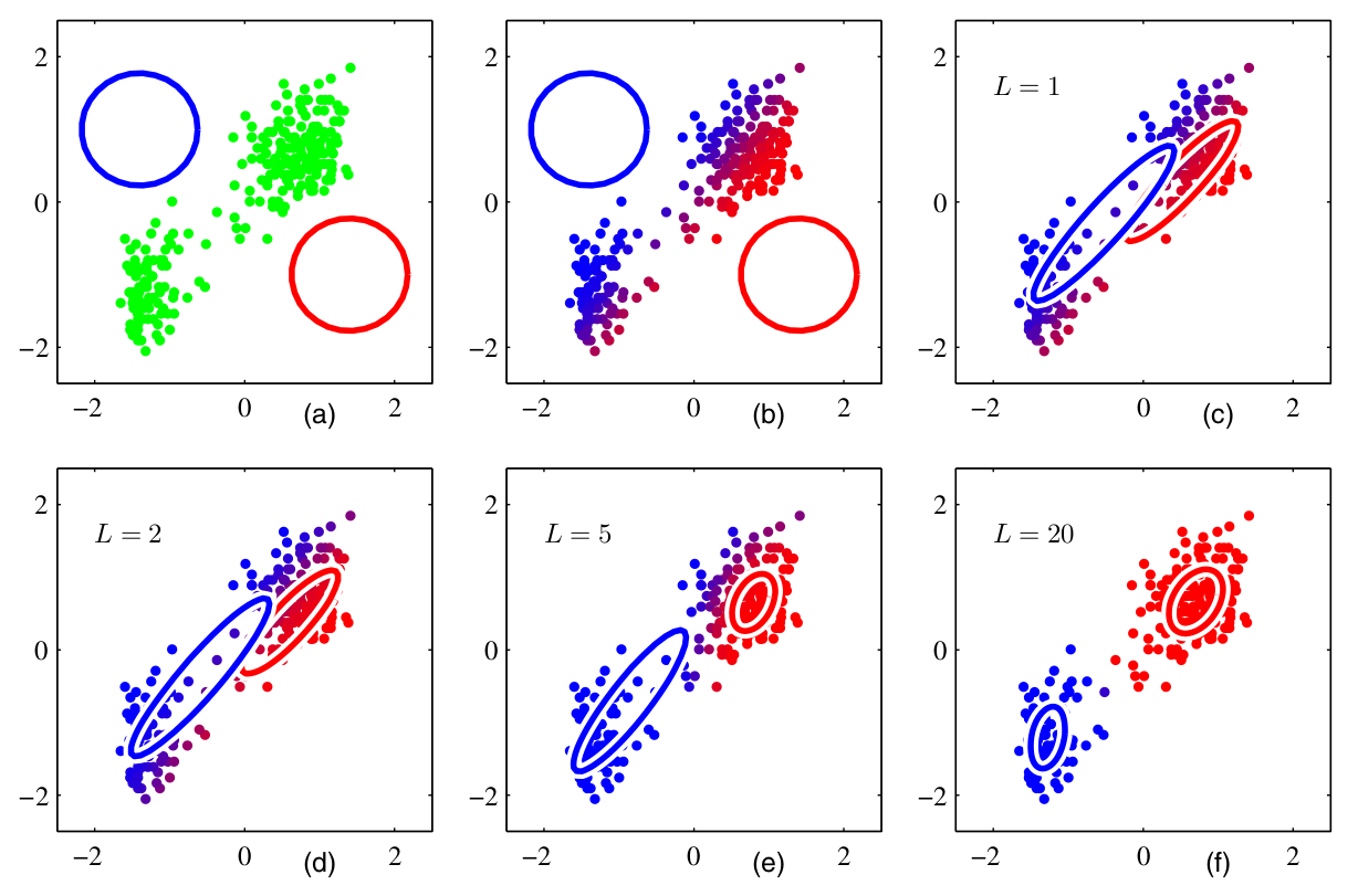
Fig. 2.3 EM algorithm for a GMM with \(K=2\) (Source: [Bishop, 2006], Section 9.2).#
There is an iterative algorithm that can solve the maximum likelihood problem by alternating between two steps. The algorithm goes as follows:
Guess the number of modes \(K\)
Randomly initialize the means \(\mu_k\), covariances \(\Sigma_k\), and mixing coefficients \(\pi_k\), and evaluate the likelihood
(E-step). Evaluate \(w_k^{(i)}\) assuming constant \(\pi, \mu, \Sigma\) (see Eq. (2.29) after the algorithm)
(2.26)#\[w_k^{(i)} := p(z^{(i)}=k| x^{(i)}, \pi, \mu, \Sigma).\](M-step). Update the parameters by solving the maximum likelihood problems for fixed \(z_k\) values.
(2.27)#\[\begin{split}\begin{aligned} \pi_k &:= \frac{1}{m}\sum_{i=1}^m w_k^{(i)} \\ \mu_k &:= \frac{\sum_{i=1}^{m} w_k^{(i)}x^{(i)}}{\sum_{i=1}^{m} w_k^{(i)}} \\ \Sigma_k &:= \frac{\sum_{i=1}^{m} w_k^{(i)}(x^{(i)}-\mu_k)(x^{(i)}-\mu_k)^{\top}}{\sum_{i=1}^{m} w_k^{(i)}} \end{aligned} \end{split}\]Evaluate the log-likelihood
(2.28)#\[l(x | \pi,\mu,\Sigma) = \sum_{i=1}^{m}\ln \left\{ \sum_{k=1}^K \pi_k \mathcal{N}(x^{(i)}|\mu_k,\Sigma_k) \right\}\]and check for convergence. If not converged, return to step 2.
In the E-step, we compute the posterior probability of \(z^{(i)}_k\) given the data point \(x^{(i)}\) and the current \(\pi\), \(\mu\), \(\Sigma\) values as
The values of \(p(x^{(i)}|z^{(i)}=k, \mu, \Sigma)\) can be computed by evaluating the \(k\)th Gaussian with parameters \(\mu_k\) and \(\Sigma_k\). And \(p(z^{(i)}=k,\pi)\) is just \(\pi_k\).
Example: Iris
An example of how to apply a GMM to a version of the Iris dataset is given below.
# Adapted from: https://www.geeksforgeeks.org/gaussian-mixture-model/
import matplotlib.pyplot as plt
from sklearn import datasets
from sklearn.mixture import GaussianMixture

# Load the first two input columns of the iris dataset
iris = datasets.load_iris()
X = iris.data[:, :2]; features = iris.feature_names[:2]
Y = iris.target

# Fit a GMM model with 3 clusters
gmm = GaussianMixture(n_components=3).fit(X)
print("Num iterations of EM algorithm =", gmm.n_iter_) # around 8
Yhat = gmm.predict(X)

# Plot the true vs learned clusters
fig, ax = plt.subplots(1, 2, figsize=(12, 5))
ax[0].scatter(X[:,0], X[:,1], c=Y); ax[0].set_title('True clusters')
ax[1].scatter(X[:,0], X[:,1], c=Yhat); ax[1].set_title('Learned clusters')
ax[0].set_xlabel(features[0]); ax[0].set_ylabel(features[1])
ax[1].set_xlabel(features[0]); ax[1].set_ylabel(features[1])
plt.show()
This leads to the following learned clusters:
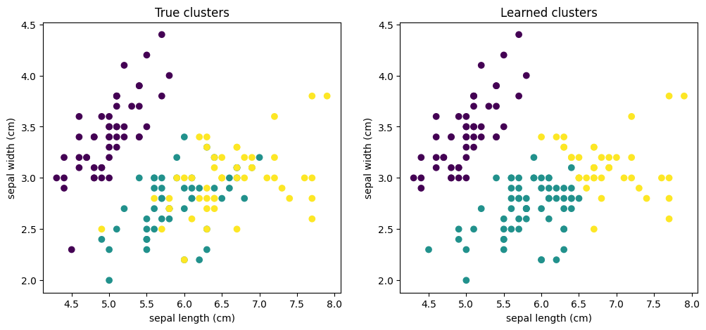
Fig. 2.4 Iris clusters with \(K=3\).#
Exercise: derive the M-step update equations following the maximum likelihood approach.
Hint: look at [Bishop, 2006], Section 9.2.
2.2.2. Applications and Limitations#
Once we have fitted a GMM on \(p(x)\), we can use it for:
Sampling: there are efficient ways to draw samples from the Gaussian distribution.
Density estimation: by evaluating the probability \(p(\tilde{x})\) of a new point \(\tilde{x}\), we can compute how probable it is that this point comes from the same distribution as the training data.
Clustering: so far we have talked about density estimation, but GMMs are typically used for clustering. Given a new query point \(\tilde{x}\), we can evaluate each of the \(K\) Gaussians and scale their probability by the respective \(\pi_k\). These will be the probabilities of \(\tilde{x}\) to be part of cluster \(k\).
Most limitations of this approach arise from the assumption that the individual clusters follow the Gaussian distribution:
If the data does not follow a Gaussian distribution, e.g. heavy-tailed distribution with outliers, then too much weight will be given to the outliers.
If there is an outlier, eventually one mode will focus only on this one data point. But if a Gaussian describes only one data point, then its variance will be zero and we recover a singularity/Dirac function.
The choice of \(K\) is crucial, and this parameter needs to be optimized in an outer loop.
GMMs do not scale well to high dimensions.
2.3. Further References#
2.3.1. Probability Theory#
[Bishop, 2006], Chapters 1 and 2, and Appendix B
[Murphy, 2022], Chapters 2 and 3
[Ng, 2022], Section 3.1 - the exponential family
2.3.2. Gaussian Mixture Models#
[Ng, 2022], Chapter 11 - main GMM reference
[Bishop, 2006], Section 9.2 - detailed derivations
Video with more visual intuition