3. Bayesian methods#
Learning outcome
How is Monte Carlo integration different than Riemannian integration? When is the former the preferred one and why?
Give two examples of sampling methods from unnormalized distributions, and sketch how they work, including strengths and weaknesses.
What is Bayesian inference and how is it useful?
Sketch the steps it takes to obtain a probabilistic answer to a (Bayesian) regression problem.
We start by introducing Bayesian statistics and the closely related sampling methods, e.g. Markov Chain Monte Carlo (MCMC). We then present Bayesian inference and its applications to regression and classification.
Notation alert: This section and the two consecutive sections (Sampling Methods and Bayesian Inference) are aligned with the notation from [Bolstad, 2009] and use \(y\) to denote the data, including both inputs and outputs. Thus, \(y\) is not the model output. From the Bayesian Linear Models section, we switch to the notation from [Murphy, 2022], i.e., using \(y\) to denote the model outputs.
3.1. Bayesian Statistics#
The main ideas upon which Bayesian statistics is founded are:
Uncertainty over parameters \(\rightarrow\) treatment as random variables
A probability over a parameter essentially expresses a degree of belief
Inference over parameters using rules of probability
We combine the prior knowledge and the observed data with Bayes’ theorem
Refresher: Bayes’ theorem is given by \(\mathbb{P}(A|B) = \frac{\mathbb{P}(B|A)\mathbb{P}(A)}{\mathbb{P}(B)}\)
So what we are interested in is the posterior distribution over our parameters, which can be found using Bayes’ theorem. While this may at first glance look straightforward and holds for the unscaled posterior, i.e., the distribution which has not been normalized by dividing by \(\mathbb{P}(B)\), obtaining the scaled posterior is much much harder due to the difficulty in computing the divisor \(\mathbb{P}(B)\). To evaluate this divisor, we often rely on Monte Carlo sampling.
What is a scaled posterior? A scaled posterior is a distribution whose integral over the entire distribution evaluates to 1.
Taking Bayes’ theorem and using the probability theorems in their conditional form, we then obtain the following formula for the posterior density
with data \(y\), parameters as random variable \(\theta\), prior \(g(\theta)\), likelihood \(f(y|\theta)\), and posterior \(g(\theta|y)\). If we now seek to compute the denominator (aka evidence), then we have to compute the integral
This integration may be very difficult and is, in most practical cases, infeasible.
3.1.1. Monte Carlo Integration#
Luckily, we do not necessarily need to compute the denominator because it is independent of \(\theta\) and thus represents a constant scaling factor not relevant for the shape of the distribution \(g(\theta|y)\). Computational Bayesian statistics relies on Monte Carlo samples from the posterior \(g(\theta | y)\), which does not require knowing the denominator of the posterior.
What we actually care about is making predictions about the output of a model \(h_{\theta}(x)\), whose parameters \(\theta\) are random variables. Without loss of generality, we can rewrite \(h_{\theta}(x)\) to \(h_x(\theta)\) as a function of the random variable \(\theta\) evaluated at a particular \(x\) (note: we use the following notation interchangably \(h_{\theta}(x)=h_x(\theta)=h(x, \theta)\)). Then the problem can be formulated as the expectation
Recall: \(h_x(\theta)=h(x,\theta)\) is the machine learning model with parameters \(\theta\) evaluated at input \(x\). And \(g(\theta|y)\) is the probability density function defining how often \(\theta\) equals a given value. If we have the linear model \(z\approx h(x,\theta) = \theta x\) and the ultimate underlying relationship between \(x\) and \(z\) is \(z=2x\), but our dataset is corrupted with noise, it might make more sense to treat \(\theta\) as, e.g., a Gaussian random variable \(\theta\sim \mathcal{N}\mathcal(\mu,\sigma^2)\). After tuning the parameters \(\mu\) and \(\sigma\) of this distribution, we might get \(\theta\sim \mathcal{N}(2.1,0.1^2)\). Now, to compute the expected value of \(h(x',\theta)\) for a novel input \(x'\) we would have to evaluate the integral in Eq. (3.3). Note: this integral can be seen as the continuous version of the sum rule of probabilities from the GMM lecture, and integrating out \(\theta\) is called marginalization (more on that in the Gaussian Processes lecture).
To approximate this integral with Monte Carlo sampling techniques, we must draw samples from the posterior \(g(\theta|y)\). Given enough samples, this process always converges to the true value of the integral according to the Monte Carlo theorem.
The resulting Bayerian inference approach consists of the following three steps:
Generate i.i.d. random samples \(\theta^{(i)}, \; i=1,2,...,N\) from the posterior \(g(\theta|y)\).
Evaluate \(h_x^{(i)}=h_x(\theta^{(i)}), \; \forall i\).
Approximate
Example: approximating \(\pi\)
We know that the area of a circle with radius \(r=1\) is \(A_{circle}=\pi r^2=\pi\), and we also know that the area of the square enclosing this circle is \(A_{square}=(2r)^2=4\). Given the ratio of the areas \(A_{circle}/A_{square}=\pi/4\) and the geometries, estimate \(\pi\).
Solution: Let us look at the top right quadrant of the square. Adapting the three steps above to this use case leads to:
Generate \(N\) i.i.d. samples from the bivariate uniform distribution \(\theta^{(i)}\sim U([0,1]^2)\) representing \(g(\theta|y)\) from above.
Evaluate \(h^{(i)}=\mathbb{1}_{(\theta_1^2+\theta_2^2)<1}(\theta^{(i)}), \; \forall i \in N\), indicating with 1 that a point is contained in the circle, and 0 otherwise.
Approximate \(A_{circle}/A_{square}=\pi/4\) by the expectation of \(h\), i.e.

Fig. 3.1 Monte Carlo method for approximating \(\pi\) (Source: Wikipedia).#
Note: of course, we could have done the above integration using, e.g., the trapezoidal rule and discretize the domain with \(\sqrt{N}\) points along \(\theta_1\) and \(\theta_2\) to also end up with \(N\) evaluations of \(h\). This would have also worked if \(g(\theta|y)\) wasn’t the uniform distribution, in which case one could interpret the integral Eq. (3.3) as a weighted average of the values of \(h\). But this would not have worked if we knew \(g(\theta|y)\) only up to a scaling factor.
Bayesian approaches based on random Monte Carlo sampling from the posterior have several advantages for us:
Given a large enough number of samples, we are not working with an approximation but with an estimate which can be made as precise as desired (given the requisite computational budget)
Sensitivity analysis of the model becomes easier.
Monte Carlo integration converges much more favorably in high dimensions - the error of the MC estimate converges at a rate \(\mathcal{O}(1/\sqrt{N})\) which depends only on the number of samples, and not on the dimension \(d\) of the variable as in numerical integration, which converges with \(\mathcal{O}(1/N^{1/d})\) on a grid with a total of N point.
The only question left is how to sample from \(g(\theta|y)\)?
3.2. Sampling Methods#
Looking at the denominator of Eq. (3.1), we notice that it is independent of \(\theta\), and is thus only a scaling factor from the perspective of the posterior \(g(\theta|y)\). This means that the numerator contains all the information describing the shape of the posterior. Thus, if we can generate sufficiently many samples from the unnormalized posterior (i.e. numerator), then these will have the exact same distribution as the true posterior. That is why you will often see the posterior written as “proportional to the prior times likelihood”
The problem we will be trying to solve here is how to generate samples from such unnormalized distributions. We use the term target distribution to describe the distribution we want to sample from.
3.2.1. Acceptance-Rejection Sampling#
Acceptance-rejection sampling draws its random samples directly from the target posterior distribution. As we only have access to the unscaled target distribution, we will have to draw from it. The acceptance-rejection algorithm is specially made for this scenario. The algorithm draws random samples from an easier-to-sample starting/candidate distribution and then selectively accepts candidate values into the final sample. For this approach to work, the candidate distribution \(g_{0}(\theta)\) has to dominate the posterior distribution, i.e. there must exist an \(M\) s.t.
Fig. 3.2 shows a candidate density for an unscaled target. It would take \(M\approx 5\) to reach a “dominance” of the candidate distribution over the target distribution.
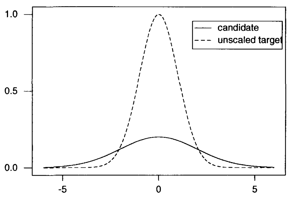
Fig. 3.2 Acceptance-rejection candidate and target distributions (Source: [Bolstad, 2009]).#
To then apply acceptance-rejection sampling to the posterior distribution, we can write out the algorithm as follows:
Draw \(N\) random samples \(\theta_{i}\) from the starting density \(g_{0}(\theta)\).
Evaluate the unscaled target density at each random sample.
Evaluate the candidate density at each random sample, and multiply by \(M\).
Compute the weights for each random sample
(3.8)#\[ w_{i} = \frac{g(\theta_{i}) \times f(y_{1}, \ldots, y_{n}| \theta_{i})}{M \times g_{0}(\theta_{i})}.\]Draw \(N\) samples from the uniform distribution \(U(0, 1)\).
If \(u_{i} < w_{i}\) accept \(\theta_{i}\).
3.2.2. Sampling-Importance-Resampling / Bayesian Bootstrap#
The sampling-importance-resampling algorithm is a two-stage extension of the acceptance-rejection sampling with improved weight calculation, but most importantly, it employs a resampling step. This resampling step resamples from the space of parameters. The weight is then calculated as
The algorithm to sample from the posterior distribution is then:
Draw \(N\) random samples \(\theta_{i}\) from the starting density \(g_{0}(\theta)\).
Calculate the value of the unscaled target density at each random sample.
Calculate the starting density at each random sample, and multiply by \(M\).
Calculate the ratio of the unscaled posterior to the starting distribution
(3.10)#\[r_{i} = \frac{g(\theta_{i})f(y_{1}, \ldots, y_{n}| \theta_{i})}{g_{0}(\theta_{i})}.\]Calculate the importance weights
(3.11)#\[w_{i} = \frac{r_{i}}{\sum r_{i}}.\]Draw \(n \leq 0.1 \times N\) random samples with the sampling probabilities given by the importance weights.
3.2.3. Adaptive Rejection Sampling#
If we cannot find a candidate/starting distribution that dominates the unscaled posterior distribution immediately, then we have to rely on adaptive rejection sampling.
This approach only works for a log-concave posterior! Log-concave means that the second derivative of the log of a log-concave density is always non-positive.
See below for an example of a log-concave distribution.
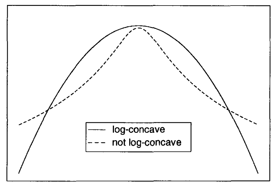
Fig. 3.3 (Not) log-concave function (Source: [Bolstad, 2009]).#
Using the tangent method, our algorithm then takes the following form:
Construct an upper bound from piecewise exponential functions, which dominate the log-concave unscaled posterior
With the envelope giving us the initial candidate density, we draw \(N\) random samples
Apply rejection sampling, see the preceding two subsections for details.
If rejected, add another exponential piece that is tangent to the target density.
As all three presented sampling approaches have their limitations, practitioners often rely on Markov chain Monte Carlo methods such as Gibbs sampling and Metropolis-Hastings.
3.2.4. Markov Chain Monte Carlo#
The idea of Markov Chain Monte Carlo (MCMC) is to construct an ergodic Markov chain of samples \(\{\theta^0, \theta^1, ...,\theta^N\}\) distributed according to the posterior distribution \(g(\theta|y) \propto g(\theta)f(y|\theta)\). This chain evolves according to a transition kernel given by \(q(\theta_{next}|\theta_{current})\). Let’s look at one of the most popular MCMC algorithms: Metropolis-Hastings.
3.2.4.1. Metropolis-Hastings#
The general Metropolis-Hastings prescribes a rule which guarantees that the constructed chain is representative of the target distribution \(g(\theta|y)\). This is done by following the algorithm:
Start at an initial point \(\theta_{current} = \theta^0\).
Sample \(\theta' \sim q(\theta_{next}|\theta_{current})\)
Compute the acceptance probability
(3.12)#\[\alpha = min \left\{ 1, \frac{g(\theta'|y) q(\theta_{current}|\theta')}{g(\theta_{current}|y) q(\theta'|\theta_{current})} \right\}\]Sample \(u\sim \text{Uniform}(0,1)\)
Set \(\theta_{\text{current}} \begin{cases} \theta' & \alpha>u \\ \theta_{\text{current}} & \text{else}\end{cases}\)
Repeat \(N\) times from step 1.
A particular choice of \(q(\cdot | \cdot)\) is, for example, the normal distribution \(\mathcal{N}(\cdot | \theta_{current}, \sigma^2)\), which results in the so-called Random Walk Metropolis algorithm. Other special cases include the Metropolis-Adjusted Langevin Algorithm (MALA), as well as the Hamiltonian Monte Carlo (HMC) algorithm.
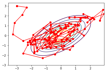
Fig. 3.4 Metropolis-Hastings trajectory (Source: relguzman.blogpost.com).#
In summary:
The unscaled posterior \(g(\theta|y) \propto g(\theta)f(y|\theta)\) contains the shape information of the posterior
For the true posterior, the unscaled posterior needs to be divided by an integral over the whole parameter space.
Integral has to be evaluated numerically, for which we rely on the Monte Carlo sampling techniques that were just presented.
3.3. Bayesian Inference#
In the Bayesian framework, everything centers around the posterior distribution and our ability to relate our previous knowledge with newly gained evidence to the next stage of our belief (of a probability distribution). With the posterior being our entire inference about the parameters given the data, multiple inference approaches exist with their roots in frequentist statistics.
3.3.1. Bayesian Point Estimation#
Bayesian point estimation chooses a single value to represent the entire posterior distribution. Potential choices here are locations like the posterior mean and posterior median. The posterior mean \(\hat{\theta}\) minimizes the posterior mean squared error
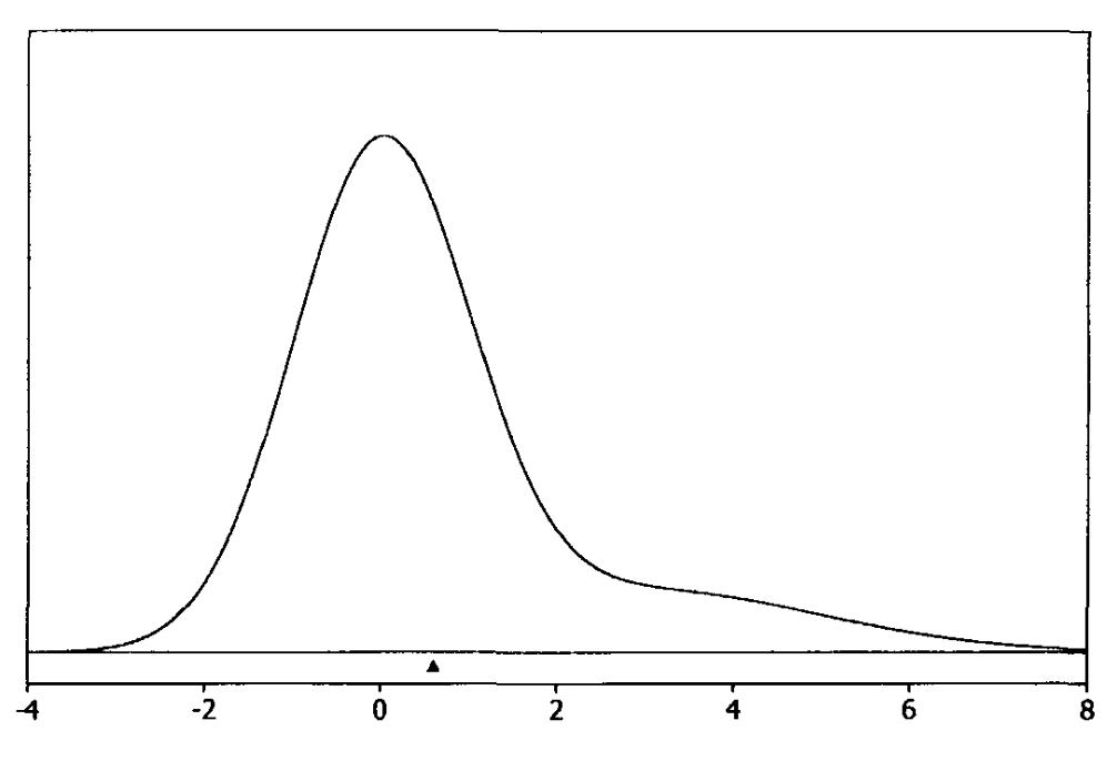
Fig. 3.5 Posterior mean (Source: [Bolstad, 2009], Chapter 3).#
And the posterior median \(\tilde{\theta}\) minimizes the posterior mean absolute deviation
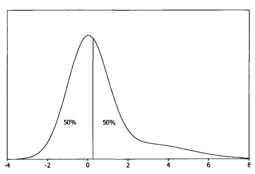
Fig. 3.6 Posterior median (Source: [Bolstad, 2009], Chapter 3).#
Another point estimate is given by the maximum a-posteriory (MAP) estimate \(\theta_{MAP}\), which is a generalization over the maximum likelihood estimate (MLE) in the sense that MAP entails a prior \(g(\theta)\).
If the prior \(g(\theta)\) is uniform (aka uninformative prior), then the MLE and MAP estimates coincide. But as soon as we have some prior knowledge about the problem, the prior regularizes the maximization problem. More on regularization in the lecture on Tricks of Optimization.
3.3.2. Bayesian Interval Estimation#
Another type of Bayesian inference is the one in which we seek to find an interval that, with a pre-determined probability, contains the true value. In Bayesian statistics, these are called credible intervals. The can be estimated by finding the interval with equal tail areas to both sides (lower \(\theta_{l}\), and upper \(\theta_{u}\)), and which has the probability \(1-\alpha\) to contain the true value of the parameter, i.e.
which we then only need to solve. A visual example of such a scenario is in the following picture:
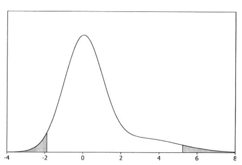
Fig. 3.7 The 95% credible interval (Source: [Bolstad, 2009], Chapter 3).#
3.3.3. Predictive Distribution of a New Observation#
If we obtain a new observation, then we can compute the updated predictive distribution by combining the conditional distribution of the new observation and conditioning it on the previous observations. Then we only need to integrate the parameter out of the joint posterior, i.e., marginalize it.
3.3.4. Bayesian Inference from a Posterior Random Sample#
When we only have a random sample from the posterior instead of a numerical approximation of the posterior, we can still apply the same techniques (i.e., point and interval estimates) but just apply them to the posterior sample.
The generated sample only constitutes an approximation, but given the sampling budget, this approximation can be made as accurate as desired. In summary, Bayesian inference can be condensed to the following main take-home knowledge:
The posterior distribution is the current summary of beliefs about the parameter in the Bayesian framework.
Bayesian inference is then performed using the probabilities calculated from the posterior distribution of the parameter.
To get an approximation of the scaling factor for the posterior, we have to utilize sampling-based Monte Carlo techniques to approximate the requisite integral.
3.4. Bayesian Linear Models#
If we are faced with the scenario of having very little data, then we ideally seek to quantify the uncertainty of our model and preserve the predictive utility of our machine learning model. The right approach to this is to extend Linear Regression and Logistic Regression with the just presented Bayesian Approach utilizing Bayesian Inference.
3.4.1. Bayesian Logistic Regression#
If we now want to capture the uncertainty over our logistic regression predictions, then we have to resort to the Bayesian approach. To make the Bayesian approach work for logistic regression, we choose to apply something called the Laplace Approximation in which we approximate the posterior using a Gaussian
where \(\omega\) corresponds to the learned parameters \(\theta\), \(\hat{\omega}\) is the MAP estimate of \(\theta\), and \(H^{-1}\) is the inverse of the Hessian (i.e., matrix of second derivatives of the negative log-posterior w.r.t. \(\omega\)) computed at \(\hat{\omega}\). Many different modes exist that represent viable solutions for this problem when we seek to optimize it.
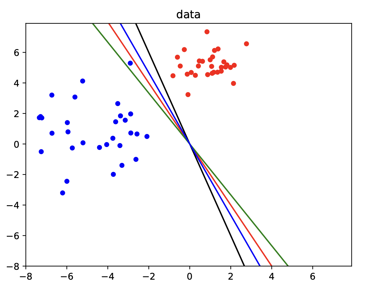
Fig. 3.8 Bayesian logistic regression data (Source: [Murphy, 2022], Chapter 10).#
In practical applications, we are interested in predicting the output \(y\) given an input \(x\). Thus, we need to compute the posterior predictive distribution
To now compute the uncertainty in our predictions, we perform a Monte Carlo Approximation of the integral using \(S\) samples from the posterior \(\omega_s \sim p(\omega|\mathcal{D})\) as
Below we look at a larger visual example of Bayesian Logistic Regression.
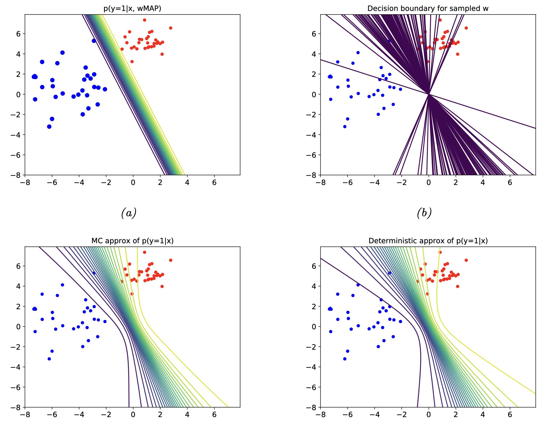
Fig. 3.9 Bayesian logistic regression (Source: [Murphy, 2022], Chapter 10).#
3.4.2. Bayesian Linear Regression#
To now introduce the Bayesian approach to linear regression, we assume that we already know the variance \(\sigma^{2}\), so the posterior which we actually want to compute at that point is
where \(\mathcal{D} = \left\{ (x_{n}, y_{n}) \right\}_{n=1:N}\). For simplicity, we assume a Gaussian prior distribution
and a likelihood is given by the Multivariate-Normal distribution
The posterior can then be analytically derived using Bayes’ rule for Gaussians (see [Murphy, 2022], Eq. 3.37) to
where \(\hat{\omega}\) is the posterior mean, and \(\hat{\Sigma}\) is the posterior covariance. A good visual example of this is the sequential Bayesian inference on a linear regression model shown below.
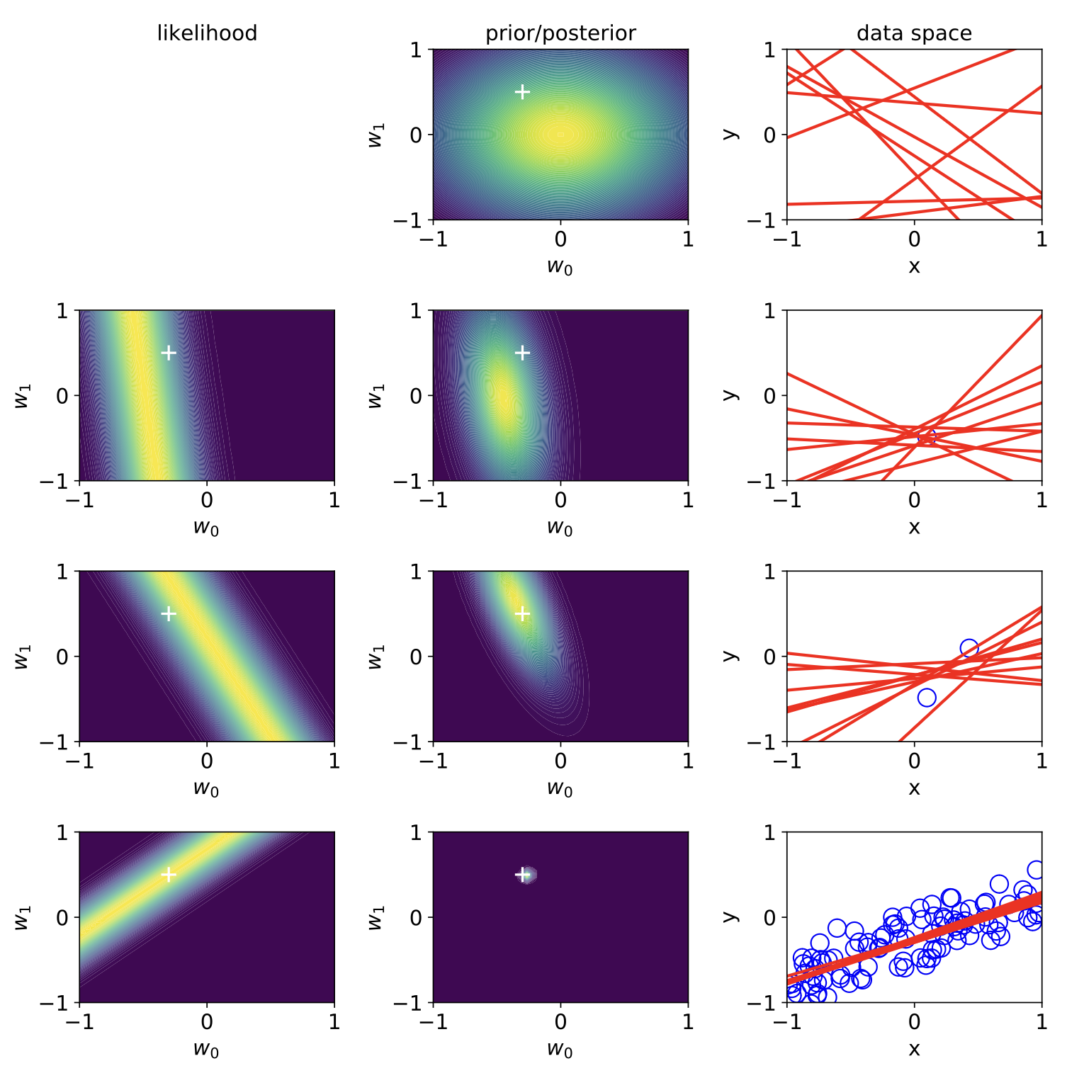
Fig. 3.10 Bayesian linear regression (Source: [Murphy, 2022], Chapter 11).#
3.5. Bayesian Machine Learning#
Let’s consider the setup we have encountered so far in which we have inputs \(x\), hyperparameters \(\theta\), and seek to predict labels \(y\). Probabilistically expressed, this amounts to \(p(y|x, \theta)\). Then the posterior is defined as \(p(\theta| \mathcal{D})\), where \(\mathcal{D}\) is our labeled dataset \(\mathcal{D} = \left\{ (x_{n}, y_{n}) \right\}_{n=1:N}\). Applying the previously discussed Bayesian approaches to these problems and the respective model parameters is called Bayesian Machine Learning.
While we lose computational efficiency at first glance, as we have to perform a sampling-based inference procedure, we gain a principled approach to discussing uncertainties within our model. This can help us most, especially when we move in the small-data limit, where we can not realistically expect our model to converge. See e.g. below a Bayesian logistic regression example in which the posterior distribution is visualized.
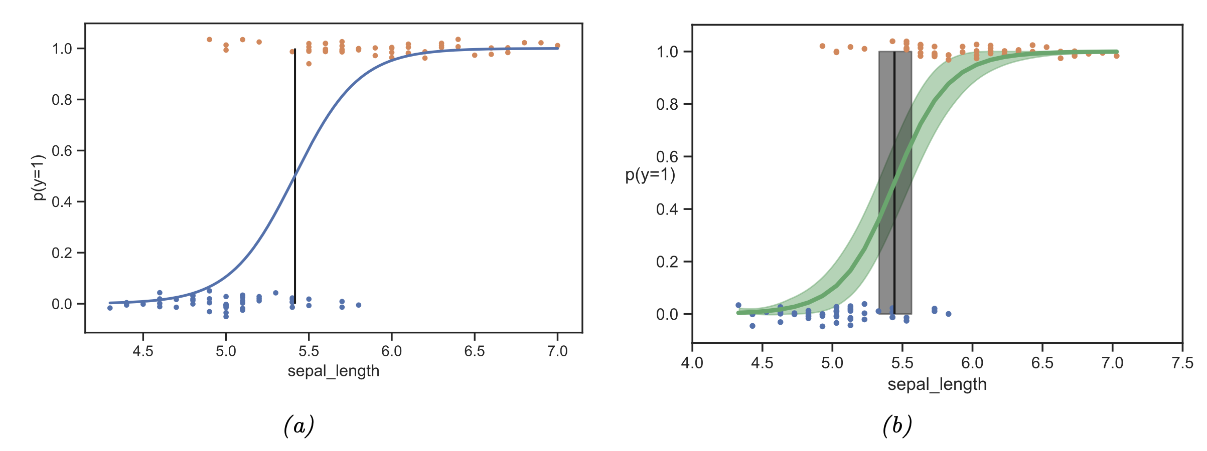
Fig. 3.11 Bayesian machine learning (Source: [Murphy, 2022], Chapter 4).#
3.6. Further References#
Bayesian Methods
There exist a vast number of references to the presented Bayesian approach, most famously the introductory treatment of Probabilistic Programming frameworks, which utilize the presented modeling approach to obtain posteriors over programs.
In addition, there exists highly curated didactic material from Michael Betancourt:
Sampling: Section 3, 4, and 5
Markov Chain Monte Carlo: Section 1, 2, and 3
Bayesian Statistics
[Bolstad, 2009], Chapters 2
Sampling
[Bolstad, 2009], Chapters 2, 5, and 6 - all presented sampling methods and background
[Robert and Casella, 2004] - deeper dive into MCMC
Bayesian Inference
[Bolstad, 2009], Chapters 3
Bayesian Regression / Classification
-
Section 10.5 on Bayesian logistic regression
Section 11.7 on Bayesian linear regression